Page 47 - Electrical Properties of Materials

30 The electron as a wave

U(Z)
ΔZ

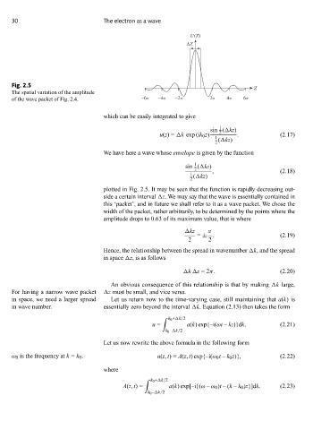
Fig. 2.5
Z
The spatial variation of the amplitude
of the wave packet of Fig. 2.4. −6π −4π −2π 2π 4π 6π

which can be easily integrated to give

1
sin ( kz)
u(z)= k exp (ik 0 z) 2 . (2.17)
1 ( kz)
2
We have here a wave whose envelope is given by the function
1
sin ( kz)
2
1 ( kz) , (2.18)
2
plotted in Fig. 2.5. It may be seen that the function is rapidly decreasing out-
side a certain interval z. We may say that the wave is essentially contained in
this ‘packet’, and in future we shall refer to it as a wave packet. We chose the
width of the packet, rather arbitrarily, to be determined by the points where the
amplitude drops to 0.63 of its maximum value, that is where
kz π
= ± . (2.19)
2 2
Hence, the relationship between the spread in wavenumber k, and the spread
in space z, is as follows
k z =2π. (2.20)

An obvious consequence of this relationship is that by making k large,
For having a narrow wave packet z must be small, and vice versa.
in space, we need a larger spread Let us return now to the time-varying case, still maintaining that a(k)is
in wave number. essentially zero beyond the interval k. Equation (2.13) then takes the form
k 0 + k/2
u = a(k)exp{–i(ωt – kz)}dk. (2.21)
k 0 – k/2

Let us now rewrite the above formula in the following form

ω 0 is the frequency at k = k 0 . u(z, t)= A(z, t)exp{–i(ω 0 t – k 0 z)}, (2.22)
where

k 0 + k/2
A(z, t)= a(k)exp[–i{(ω – ω 0 )t –(k – k 0 )z}]dk. (2.23)
k 0 – k/2