Page 64 - Electrical Properties of Materials

The uncertainty relationship 47

1
V 1 2
r.h.s.

1
0.75V 2
1

1
0.50V 2
1
l.h.s.
1
0.25V 2
1
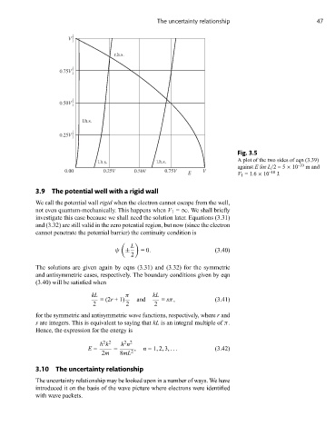
Fig. 3.5
l.h.s. l.h.s. A plot of the two sides of eqn (3.39)
against E for L/2=5 × 10 –10 mand
0.00 0.25V 0.50V 0.75V E V V 1 = 1.6 × 10 –18 J.

3.9 The potential well with a rigid wall
We call the potential wall rigid when the electron cannot escape from the well,
not even quantum-mechanically. This happens when V 1 = ∞. We shall briefly
investigate this case because we shall need the solution later. Equations (3.31)
and (3.32) are still valid in the zero potential region, but now (since the electron
cannot penetrate the potential barrier) the continuity condition is

L

ψ ± = 0. (3.40)
2
The solutions are given again by eqns (3.31) and (3.32) for the symmetric
and antisymmetric cases, respectively. The boundary conditions given by eqn
(3.40) will be satisfied when
kL π kL
=(2r +1) and = sπ, (3.41)
2 2 2
for the symmetric and antisymmetric wave functions, respectively, where r and
s are integers. This is equivalent to saying that kL is an integral multiple of π.
Hence, the expression for the energy is
2 2
2 2
k h n
E = = , n = 1,2,3, ... (3.42)
2m 8mL 2
3.10 The uncertainty relationship

The uncertainty relationship may be looked upon in a number of ways. We have
introduced it on the basis of the wave picture where electrons were identified
with wave packets.