Page 75 - Electrical Properties of Materials

58 The hydrogen atom and the periodic table

a free electron; so it is less strongly bound to the proton. If it is less strongly
bound, it can wander farther away; so the radius corresponding to maximum
probability increases.

4.2 Quantum numbers
So much about spherically symmetrical solutions. The general solution in-
cludes, of course, our previously obtained solutions, denoted by R(r) from here
on but shows variations in θ and φ as well. It can be written as
m l
(r, θ, φ)= R nl (r)Y (θ, φ). (4.27)
We have met n before; l and m l ψ n,l,m l l
represent two more discrete sets
of constants which ensure that the It may be shown (alas, not by simple means) from the original differential
solutions have physical meaning. equation (eqn (4.12)) that the quantum numbers must satisfy the following
These discrete sets of constants al- relationships
ways appear in the solutions of n = 1,2,3 ...
partial differential equations; you
may remember them from the l = 0,1,2, ... n –1 (4.28)
problems of the vibrating string or m l =0, ±1, ±2 ... ± l.
of the vibrating membrane. They
are generally called eigenvalues;
For n = 1 there is only one possibility: l = 0 and m l = 0, and the corres-
in quantum mechanics they are re-
ponding wave function is the one we guessed in eqn (4.13). For the spherically
ferred to as quantum numbers.
symmetrical case the wave functions have already been plotted for n = 1,2,3;
now let us see a wave function which is dependent on direction. Choosing n =2,
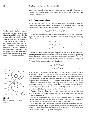
l =1, m l = 0, the corresponding wave function is
0
ψ 210 = R 21 (r)Y (θ, φ)
1
= re –c 0 r/2 cos θ. (4.29)
5
c z
0
This equation tells us how the probability of finding the electron varies as
3
a function of r and θ. Thus, the equal-probability surfaces may be determ-
ined. The spherical symmetry has gone, but there is still cylindrical symmetry
1 (no dependence on φ). It is therefore sufficient to plot the curves in, say, the
2
|ψ| = 0.9, 0.5, 0.2 xz-plane. This is done in Fig. 4.4, where the unit of distance is taken as one

–1 Bohr radius, and the maximum probability (at x = 0 and z = ±2/c 0 ) is nor-
malized to unity. It can be clearly seen that the θ = 0 and θ = π directions are
preferred (which of course follows from eqn (4.29) directly); there is a higher
–3 probability of finding the electron in those directions.
With n = 2 and l = 1 there are two more states, but they give nothing new.
The preferential directions in those cases are in the direction of the ±x and
–5
–4 –2 0 2 c x 4 ±y-axes, respectively.
0
For higher values of n and l the equal-probability curves look more and
Fig. 4.4
2
Plots of constant |ψ 210 | in the more complicated. Since at this level of treatment they will not add much to
xz-plane. our picture of the hydrogen atom, we can safely omit them.
I have to add a few words about notations. However convenient the para-
meters n and l might appear, they are never (or at least very rarely) used in that
form. The usual notation is a number, equal to the value of n,followedbya
letter, which is related to l by the following rule