Page 133 - Electromagnetics

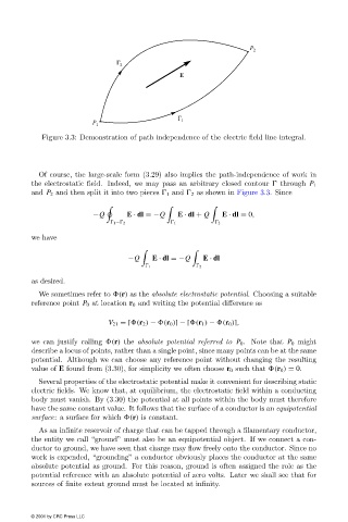
Figure 3.3: Demonstration of path independence of the electric field line integral.

Of course, the large-scale form (3.29)also implies the path-independence of work in
the electrostatic field. Indeed, we may pass an arbitrary closed contour through P 1
and P 2 and then split it into two pieces 1 and 2 as shown in Figure 3.3. Since

−Q E · dl =−Q E · dl + Q E · dl = 0,
1 − 2 1 2
we have

−Q E · dl =−Q E · dl
1 2
as desired.
We sometimes refer to (r) as the absolute electrostatic potential. Choosing a suitable
reference point P 0 at location r 0 and writing the potential difference as

V 21 = [ (r 2 ) − (r 0 )] − [ (r 1 ) − (r 0 )],

we can justify calling (r) the absolute potential referred to P 0 . Note that P 0 might
describe a locus of points, rather than a single point, since many points can be at the same
potential. Although we can choose any reference point without changing the resulting
value of E found from (3.30), for simplicity we often choose r 0 such that (r 0 ) = 0.
Several properties of the electrostatic potential make it convenient for describing static
electric fields. We know that, at equilibrium, the electrostatic field within a conducting
body must vanish. By (3.30)the potential at all points within the body must therefore
have the same constant value. It follows that the surface of a conductor is an equipotential
surface: a surface for which (r) is constant.
As an infinite reservoir of charge that can be tapped through a filamentary conductor,
the entity we call “ground” must also be an equipotential object. If we connect a con-
ductor to ground, we have seen that charge may flow freely onto the conductor. Since no
work is expended, “grounding” a conductor obviously places the conductor at the same
absolute potential as ground. For this reason, ground is often assigned the role as the
potential reference with an absolute potential of zero volts. Later we shall see that for
sources of finite extent ground must be located at infinity.

© 2001 by CRC Press LLC