Page 135 - Electromagnetics

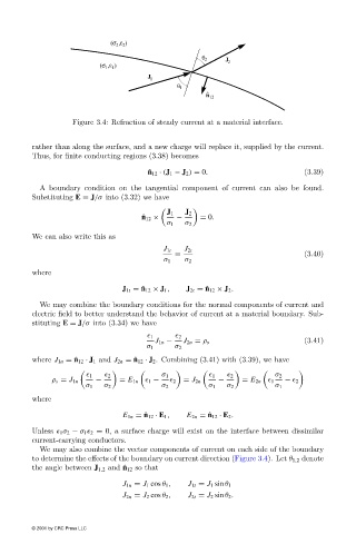
Figure 3.4: Refraction of steady current at a material interface.

rather than along the surface, and a new charge will replace it, supplied by the current.
Thus, for finite conducting regions (3.38)becomes
ˆ n 12 · (J 1 − J 2 ) = 0. (3.39)

A boundary condition on the tangential component of current can also be found.
Substituting E = J/σ into (3.32)we have

J 1 J 2
ˆ n 12 × − = 0.
σ 1 σ 2
We can also write this as
J 1t J 2t
= (3.40)
σ 1 σ 2
where
J 1t = ˆ n 12 × J 1 , J 2t = ˆ n 12 × J 2 .

We may combine the boundary conditions for the normal components of current and
electric field to better understand the behavior of current at a material boundary. Sub-
stituting E = J/σ into (3.34)we have
1 2
J 1n − J 2n = ρ s (3.41)
σ 1 σ 2
where J 1n = ˆ n 12 · J 1 and J 2n = ˆ n 12 · J 2 . Combining (3.41)with (3.39), we have

1 2 σ 1 1 2 σ 2
ρ s = J 1n − = E 1n 1 − 2 = J 2n − = E 2n 1 − 2
σ 1 σ 2 σ 2 σ 1 σ 2 σ 1
where

E 1n = ˆ n 12 · E 1 , E 2n = ˆ n 12 · E 2 .

Unless 1 σ 2 − σ 1 2 = 0, a surface charge will exist on the interface between dissimilar
current-carrying conductors.
We may also combine the vector components of current on each side of the boundary
to determine the effects of the boundary on current direction (Figure 3.4). Let θ 1,2 denote
the angle between J 1,2 and ˆ n 12 so that
J 1n = J 1 cos θ 1 , J 1t = J 1 sin θ 1
J 2n = J 2 cos θ 2 , J 2t = J 2 sin θ 2 .

© 2001 by CRC Press LLC