Page 148 - Electromagnetics

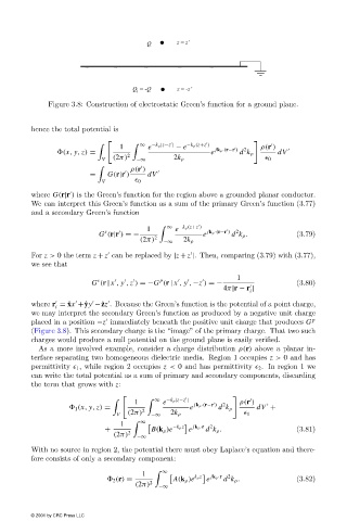
Figure 3.8: Construction of electrostatic Green’s function for a ground plane.

hence the total potential is

∞ −k ρ |z−z | −k ρ (z+z )
1 e − e jk ρ ·(r−r ) 2 ρ(r )
(x, y, z) = 2 e d k ρ dV
V (2π) −∞ 2k ρ 0
ρ(r )

= G(r|r ) dV
V 0

where G(r|r ) is the Green’s function for the region above a grounded planar conductor.
We can interpret this Green’s function as a sum of the primary Green’s function (3.77)
and a secondary Green’s function

1 ∞ e −k ρ (z+z )

s jk ρ ·(r−r ) 2
G (r|r ) =− 2 e d k ρ . (3.79)
(2π) 2k ρ
−∞
For z > 0 the term z + z can be replaced by |z + z |. Then, comparing (3.79)with (3.77),

we see that
1
s p
G (r | x , y , z ) =−G (r | x , y , −z ) =− (3.80)

4π|r − r |
i

where r = ˆ xx + ˆ yy − ˆ zz . Because the Green’s function is the potential of a point charge,
i
we may interpret the secondary Green’s function as produced by a negative unit charge
placed in a position −z immediately beneath the positive unit charge that produces G p

(Figure 3.8). This secondary charge is the “image” of the primary charge. That two such
charges would produce a null potential on the ground plane is easily verified.
As a more involved example, consider a charge distribution ρ(r) above a planar in-
terface separating two homogeneous dielectric media. Region 1 occupies z > 0 and has
permittivity 1 , while region 2 occupies z < 0 and has permittivity 2 . In region 1 we
can write the total potential as a sum of primary and secondary components, discarding
the term that grows with z:

1 e jk ρ ·(r−r ) 2 ρ(r )
∞ −k ρ |z−z |

1 (x, y, z) = 2 e d k ρ dV +
V (2π) −∞ 2k ρ 1
1 ∞ −k ρ z jk ρ ·r 2
+ B(k ρ )e e d k ρ . (3.81)
(2π) 2 −∞
With no source in region 2, the potential there must obey Laplace’s equation and there-
fore consists of only a secondary component:
1 ∞ k ρ z jk ρ ·r 2
2 (r) = A(k ρ )e e d k ρ . (3.82)
(2π) 2
−∞
© 2001 by CRC Press LLC