Page 174 - Electromagnetics

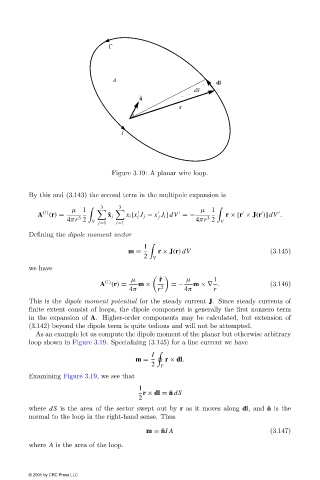
Figure 3.19: A planar wire loop.

By this and (3.143)the second term in the multipole expansion is
3 3
µ 1

µ 1

(1)
A (r) = ˆ x j x i [x J j − x J i ] dV =− r × [r × J(r )] dV .
i
j
3
3
4πr 2 V j=1 i=1 4πr 2 V
Defining the dipole moment vector
1
m = r × J(r) dV (3.145)
2 V
we have
µ ˆ r µ 1
(1)
A (r) = m × =− m ×∇ . (3.146)
4π r 2 4π r
This is the dipole moment potential for the steady current J. Since steady currents of
finite extent consist of loops, the dipole component is generally the first nonzero term
in the expansion of A. Higher-order components may be calculated, but extension of
(3.142)beyond the dipole term is quite tedious and will not be attempted.
As an example let us compute the dipole moment of the planar but otherwise arbitrary
loop shown in Figure 3.19. Specializing (3.145)for a line current we have
I
m = r × dl.
2
Examining Figure 3.19, we see that
1
r × dl = ˆ n dS
2
where dS is the area of the sector swept out by r as it moves along dl, and ˆ n is the
normal to the loop in the right-hand sense. Thus

m = ˆ nIA (3.147)
where A is the area of the loop.

© 2001 by CRC Press LLC