Page 185 - Electromagnetics

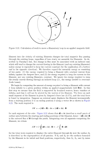
Figure 3.21: Calculation of work to move a filamentary loop in an applied magnetic field.

filament into the vicinity of existing filaments changes the total magnetic flux passing
through the existing loops, regardless of how slowly we assemble the filaments. As de-
scribed by Faraday’s law, this change in flux must be associated with an induced emf,
which will tend to change the current flowing in the filament (and any existing filaments)
unless energy is expended to keep the current constant (by the application of a battery
emf in the opposite direction). We therefore regard the assembly energy as consisting
of two parts: (1)the energy required to bring a filament with constant current from
infinity against the Ampere force, and (2)the energy required to keep the current in this
filament, and any existing filaments, constant. We ignore the energy required to keep
the steady current flowing through an isolated loop (i.e., the energy needed to overcome
Joule losses).
We begin by computing the amount of energy required to bring a filament with current
I from infinity to a given position within an applied magnetostatic field B(r). In this
first step we assume that the field is supported by localized sources, hence vanishes at
infinity, and that it will not be altered by the motion of the filament. The force on each
small segment of the filament is given by Ampere’s force law (3.171), and the total force
is found by integration. Suppose an external agent displaces the filament incrementally
from a starting position 1 to an ending position 2 along a vector δr as shown in Figure
3.21. The work required is

δW =−(Idl × B) · δr = (Idl × δr) · B

for each segment of the wire. Figure 3.21 shows that dl × δr describes a small patch of
surface area between the starting and ending positions of the filament, hence −(dl×δr)·B
is the outward flux of B through the patch. Integrating over all segments comprising the
filament, we obtain

W = I (dl × δr) · B =−I B · dS
S 0

for the total work required to displace the entire filament through δr; here the surface S 0
is described by the superposition of all patches. If S 1 and S 2 are the surfaces bounded
by the filament in its initial and final positions, respectively, then S 1 , S 2 , and S 0 taken

© 2001 by CRC Press LLC