Page 49 - Electromagnetics

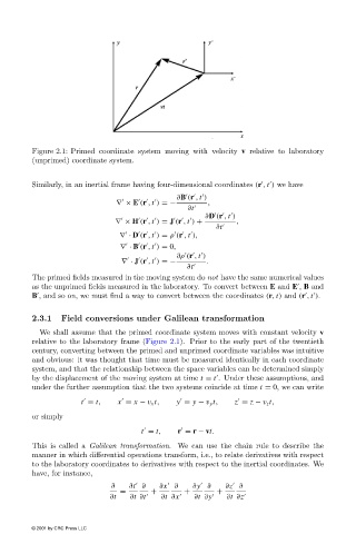
Figure 2.1: Primed coordinate system moving with velocity v relative to laboratory
(unprimed) coordinate system.

Similarly, in an inertial frame having four-dimensional coordinates (r , t ) we have

∂B (r , t )

∇ × E (r , t ) =− ,
∂t

∂D (r , t )

∇ × H (r , t ) = J (r , t ) + ,
∂t

∇ · D (r , t ) = ρ (r , t ),

∇ · B (r , t ) = 0,
∂ρ (r , t )

∇ · J (r , t ) =− .
∂t
The primed fields measured in the moving system do not have the same numerical values

as the unprimed fields measured in the laboratory. To convert between E and E , B and

B , and so on, we must find a way to convert between the coordinates (r, t) and (r , t ).
2.3.1 Field conversions under Galilean transformation
We shall assume that the primed coordinate system moves with constant velocity v
relative to the laboratory frame (Figure 2.1). Prior to the early part of the twentieth
century, converting between the primed and unprimed coordinate variables was intuitive
and obvious: it was thought that time must be measured identically in each coordinate
system, and that the relationship between the space variables can be determined simply
by the displacement of the moving system at time t = t . Under these assumptions, and

under the further assumption that the two systems coincide at time t = 0, we can write

t = t, x = x − v x t, y = y − v y t, z = z − v z t,

or simply

t = t, r = r − vt.
This is called a Galilean transformation. We can use the chain rule to describe the
manner in which differential operations transform, i.e., to relate derivatives with respect
to the laboratory coordinates to derivatives with respect to the inertial coordinates. We
have, for instance,

∂ ∂t ∂ ∂x ∂ ∂y ∂ ∂z ∂

= + + +
∂t ∂t ∂t ∂t ∂x ∂t ∂y ∂t ∂z
© 2001 by CRC Press LLC