Page 63 - Electromagnetics Handbook

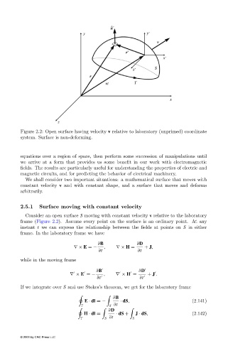
Figure 2.2: Open surface having velocity v relative to laboratory (unprimed) coordinate
system. Surface is non-deforming.

equations over a region of space, then perform some succession of manipulations until
we arrive at a form that provides us some benefit in our work with electromagnetic
fields. The results are particularly useful for understanding the properties of electric and
magnetic circuits, and for predicting the behavior of electrical machinery.
We shall consider two important situations: a mathematical surface that moves with
constant velocity v and with constant shape, and a surface that moves and deforms
arbitrarily.

2.5.1 Surface moving with constant velocity
Consider an open surface S moving with constant velocity v relative to the laboratory
frame (Figure 2.2). Assume every point on the surface is an ordinary point. At any
instant t we can express the relationship between the fields at points on S in either
frame. In the laboratory frame we have

∂B ∂D
∇× E =− , ∇× H = + J,
∂t ∂t
while in the moving frame

∂B ∂D

∇ × E =− , ∇ × H = + J .
∂t ∂t
If we integrate over S and use Stokes’s theorem, we get for the laboratory frame

∂B

E · dl =− · dS, (2.141)
S ∂t

∂D
H · dl = · dS + J · dS, (2.142)
S ∂t S

© 2001 by CRC Press LLC