Page 66 - Electromagnetics Handbook

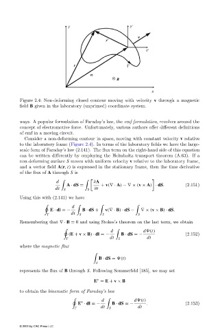
Figure 2.4: Non-deforming closed contour moving with velocity v through a magnetic
field B given in the laboratory (unprimed) coordinate system.

ways. A popular formulation of Faraday’s law, the emf formulation, revolves around the
concept of electromotive force. Unfortunately, various authors offer different definitions
of emf in a moving circuit.
Consider a non-deforming contour in space, moving with constant velocity v relative
to the laboratory frame (Figure 2.4). In terms of the laboratory fields we have the large-
scale form of Faraday’s law (2.141). The flux term on the right-hand side of this equation
can be written differently by employing the Helmholtz transport theorem (A.63). If a
non-deforming surface S moves with uniform velocity v relative to the laboratory frame,
and a vector field A(r, t) is expressed in the stationary frame, then the time derivative
of the flux of A through S is
d ∂A
A · dS = + v(∇· A) −∇ × (v × A) · dS. (2.151)
dt S S ∂t

Using this with (2.141) we have

d
E · dl =− B · dS + v(∇· B) · dS − ∇× (v × B) · dS.
dt S S S
Remembering that ∇· B = 0 and using Stokes’s theorem on the last term, we obtain
d d (t)

(E + v × B) · dl =− B · dS =− (2.152)
dt S dt
where the magnetic flux

B · dS = (t)
S
represents the flux of B through S. Following Sommerfeld [185], we may set

E = E + v × B
∗
to obtain the kinematic form of Faraday’s law

d d (t)

∗
E · dl =− B · dS =− . (2.153)
dt S dt

© 2001 by CRC Press LLC