Page 147 -

xyroots=fsolve('funname',xyguess)
xyroots =
4.7081 -1.3541

5. To find the second root, use the second value of xyguess, which
is the estimate of the other root, obtained from an examination of
the contour plot in step 1 of the fsolve command:
xyguess=[-4 2];
xyroots=fsolve('funname',xyguess)

xyroots =
-3.9081 2.9541
This method can be extended to any number of variables and nonlinear equa-
tions, but the estimate of the roots becomes much more difficult and we will
not go into further details here.

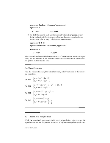
In-Class Exercises
Find the values of x and y that simultaneously satisfy each pair of the follow-
ing equations:
 z = 0 = x + 2 y 3−
3
Pb. 5.10  1 2 2
 z = 0 = x + 3 y − 4
2
 z = 0 = sin ( x + y +) y − x 27 4− /
3
2
2
Pb. 5.11  1 2 2
 z = 0 = x + 3 y − 31
2
 z = 0 = x 32 + ( y 3− ) 2 − 12
/
Pb. 5.12  1
 z = 0 = x + y 9−
2
 z = 0 = tan( ) y
x −

1
Pb. 5.13  2 y 1
x −
 z = 0 = sin ( ) 4 − 4

2
5.2 Roots of a Polynomial

While the analytical expressions for the roots of quadratic, cubic, and quartic
equations are known, in general, the roots of higher-order polynomials can-

© 2001 by CRC Press LLC