Page 277 -

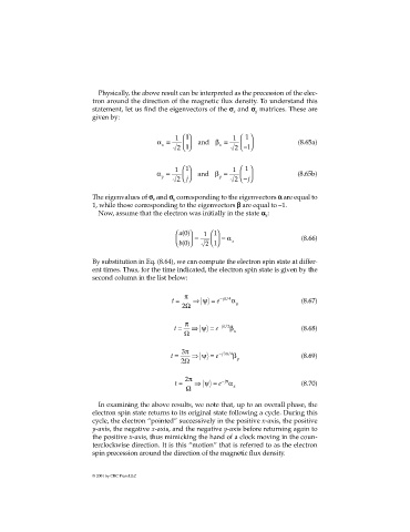
Physically, the above result can be interpreted as the precession of the elec-
tron around the direction of the magnetic flux density. To understand this
statement, let us find the eigenvectors of the σσ σσ and σσ σσ matrices. These are
y
x
given by:

α = 1   1 and β = 1  1   (8.65a)

 
x x
2   1 2  −  1
α = 1   1 and β = 1  1   (8.65b)

 
y j   y j − 
2 2 
The eigenvalues of σσ σσ and σσ σσ corresponding to the eigenvectors αα αα are equal to
x
y
1, while those corresponding to the eigenvectors ββ ββ are equal to –1.
Now, assume that the electron was initially in the state αα αα :
x
 a()0  1  
1
  =   =α x (8.66)
 b()0  2 1  
By substitution in Eq. (8.64), we can compute the electron spin state at differ-
ent times. Thus, for the time indicated, the electron spin state is given by the
second column in the list below:

π
t = ⇒ ψ = e j − π 4/ α (8.67)
2Ω y

π
t = ⇒ ψ = e j − π/2 β (8.68)
Ω x

3π
t = ⇒ ψ = e j − 3π/ 4 β (8.69)
2Ω y

2π
t = ⇒ ψ = e j − π α (8.70)
Ω x

In examining the above results, we note that, up to an overall phase, the
electron spin state returns to its original state following a cycle. During this
cycle, the electron “pointed” successively in the positive x-axis, the positive
y-axis, the negative x-axis, and the negative y-axis before returning again to
the positive x-axis, thus mimicking the hand of a clock moving in the coun-
terclockwise direction. It is this “motion” that is referred to as the electron
spin precession around the direction of the magnetic flux density.

© 2001 by CRC Press LLC