Page 94 -

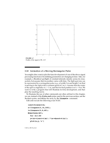
FIGURE 3.7
Profile of the signal of Pb. 3.37.

3.10 Animation of a Moving Rectangular Pulse
You might often want to plot the time development of one of the above signal
processing functions if its defining parameters are changing in time. Take, for
example, a theatrical spotlight of constant intensity density across its cross-
section, but assume that its position varies with time. The light spot size can
be represented by a rectangular pulse (e.g., of width 2 m and height 1 m) that
is moving to the right with a constant speed of 1 m/s. Assume that the center
of the spot is originally at x = 1 m, and that its final position is at x = 8 m. We
want to write a program that will illustrate its time development, and then
play the resulting movie.
To illustrate the use of other commands not often utilized in this chapter,
we can, instead of the if-else-end syntax used in the previous section, use the
Boolean syntax, and define the array by the linspace command.
Edit and execute the following script M-file:

lrect=0;hrect=2;
x=linspace(0,10,200);
t=linspace(0,8,40);
M=moviein(40);
for m=1:40
y=(x>=lrect+t(m)).*(x<=hrect+t(m));
plot(x,y,'r')

© 2001 by CRC Press LLC