Page 84 - Elements of Distribution Theory

P1: JZP
052184472Xc03 CUNY148/Severini May 24, 2005 2:34

70 Characteristic Functions

Real Part

u (t)

−
−
− −
t

Imaginary Part

v (t)

−
− − −
t
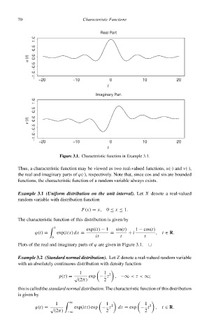
Figure 3.1. Characteristic function in Example 3.1.

Thus, a characteristic function may be viewed as two real-valued functions, u(·) and v(·),
the real and imaginary parts of ϕ(·), respectively. Note that, since cos and sin are bounded
functions, the characteristic function of a random variable always exists.

Example 3.1 (Uniform distribution on the unit interval). Let X denote a real-valued
random variable with distribution function
F(x) = x, 0 ≤ x ≤ 1.

The characteristic function of this distribution is given by
1
exp(it) − 1 sin(t) 1 − cos(t)

ϕ(t) = exp(itx) dx = = + i , t ∈ R.
0 it t t
Plots of the real and imaginary parts of ϕ are given in Figure 3.1.
Example 3.2 (Standard normal distribution). Let Z denote a real-valued random variable
with an absolutely continuous distribution with density function
1 1 2
p(z) = √ exp − z , −∞ < z < ∞;
(2π) 2
this is called the standard normal distribution. The characteristic function of this distribution
is given by
1 ∞ 1 2 1 2
ϕ(t) = √ exp(itz)exp − z dz = exp − t , t ∈ R.
(2π) −∞ 2 2