Page 87 - Academic Press Encyclopedia of Physical Science and Technology 3rd Chemical Engineering

P1: LLL Revised Pages
Encyclopedia of Physical Science and Technology EN002E-49 May 17, 2001 20:13

Batch Processing 51

and the computing time that can be spent solving each
case. The formulation of the equations that represent the
physical situation is not highly complex, but it cannot be
reduced to a routine procedure. The equations result from
the application of basic laws of physics to the various
cases. Commonly used for this purpose are the laws of
conservation of mass, energy, and momentum and several
others. The problem is determined by defining the sys-
tem being considered, the boundary conditions affecting
the system, and a balance of mass, energy, or momentum
(MEM), rates expressed by:

I − O + G = A (5)
where I is input, O output, G generation, and A accu-
mulation of MEM in the system. In certain situations the
MEM balance may have to be implemented or replaced
by equivalent physical laws. Thus, in a problem of fluid
mechanics, the basic elements of analysis are stresses and
strain rates. A force balance generates the equations of
motion; a mass balance yields the equation of continu-
ity. These balances must be implemented with the rela-
tionship between stresses and strain rates, which must be
established experimentally. When the classical approach
of balancing MEM rates [Eq. (5)] is not possible due to
complexity, the system may have to be redefined in sim-
pler terms, or a time history of the process may have to be
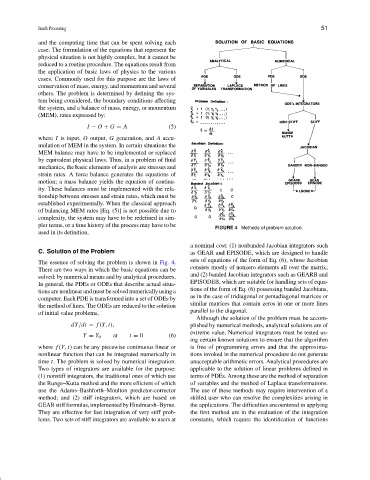
FIGURE 4 Methods of problem solution.
used in its definition.
a nominal cost: (1) nonbanded Jacobian integrators such
C. Solution of the Problem as GEAR and EPISODE, which are designed to handle
sets of equations of the form of Eq. (6), whose Jacobian
The essence of solving the problem is shown in Fig. 4.
consists mostly of nonzero elements all over the matrix;
There are two ways in which the basic equations can be
and (2) banded Jacobian integrators such as GEARB and
solved: by numerical means and by analytical procedures.
EPISODEB, which are suitable for handling sets of equa-
In general, the PDEs or ODEs that describe actual situa-
tions of the form of Eq. (6) possessing banded Jacobians,
tions are nonlinear and must be solved numerically using a
as in the case of tridiagonal or pentadiagonal matrices or
computer. Each PDE is transformed into a set of ODEs by
similar matrices that contain zeros in one or more lines
the method of lines. The ODEs are reduced to the solution
parallel to the diagonal.
of initial value problems,
Although the solution of the problem must be accom-
dY/dt = f (Y, t), plished by numerical methods, analytical solutions are of
extreme value. Numerical integrators must be tested us-
Y = Y 0 at t = 0 (6)
ing certain known solutions to ensure that the algorithm
where f (Y, t) can be any piecewise continuous linear or is free of programming errors and that the approxima-
nonlinear function that can be integrated numerically in tions invoked in the numerical procedure do not generate
time t. The problem is solved by numerical integration. unacceptable arithmetic errors. Analytical procedures are
Two types of integrators are available for the purpose: applicable to the solution of linear problems defined in
(1) nonstiff integrators, the traditional ones of which use terms of PDEs. Among these are the method of separation
the Runge–Kutta method and the more efficient of which of variables and the method of Laplace transformations.
use the Adams–Bashforth–Moulton predictor-corrector The use of these methods may require intervention of a
method; and (2) stiff integrators, which are based on skilled user who can resolve the complexities arising in
GEAR stiff formulas, implemented by Hindmarsh–Byrne. the applications. The difficulties encountered in applying
They are effective for fast integration of very stiff prob- the first method are in the evaluation of the integration
lems. Two sets of stiff integrators are available to users at constants, which require the identification of functions