Page 303 - Academic Press Encyclopedia of Physical Science and Technology 3rd Polymer

P1: GQT/MBQ P2: GPJ Final Pages
Encyclopedia of Physical Science and Technology EN014C-660 July 28, 2001 17:14

Rheology of Polymeric Liquids 241

twodifferencesofnormalstresscomponentsandoneshear
component,
N 1 = σ 11 − σ 22 , N 2 = σ 22 − σ 33 , and σ 12 , (11)

in which N 1 is called the first normal stress difference,
N 2 is called the second normal stress difference, and σ 12
is called the shear stress. Following the nomenclatures
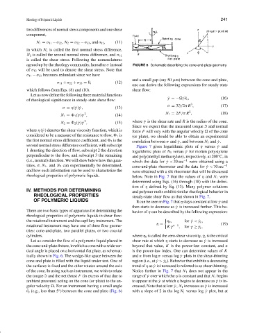
agreed up by the rheology community, hereafter σ instead FIGURE 6 Schematic describing the cone-and-plate geometry.
of σ 12 will be used to denote the shear stress. Note that
σ 11 − σ 33 becomes redundant since we have
and a small gap (say 50 µm) between the cone and plate,
σ 11 + σ 22 + σ 33 = 0, (12)
one can derive the following expressions for steady-state
which follows from Eqs. (8) and (10). shear flow:
Let us now define the following three material functions
˙ γ =− /θ c , (16)
of rheological significance in steady-state shear flow:
3
σ = 3 /2π R , (17)
σ = η( ˙γ ) ˙γ, (13)
2
2
N 1 = 1 ( ˙γ ) ˙γ , (14) N 1 = 2F/π R , (18)
2
N 2 = 2 ( ˙γ ) ˙γ , (15) where ˙γ is the shear rate and R is the radius of the cone.
Since we expect that the measured torque and normal
where η ( ˙γ ) denotes the shear viscosity function, which is force F will vary with the angular velocity of the cone
considered to be a measure of the resistance to flow, 1 is (or plate), we should be able to obtain an experimental
the first normal stress difference coefficient, and 2 is the correlation between σ and ˙γ , and between N 1 and ˙γ .
second normal stress difference coefficient, with subscript Figure 7 gives logarithmic plots of η versus ˙γ and
1 denoting the direction of flow, subscript 2 the direction logarithmic plots of N 1 versus ˙γ for molten polystyrene
perpendicular to the flow, and subscript 3 the remaining and poly(methyl methacrylate), respectively, at 200 C, in
◦
(i.e., neutral) direction. We will show below how the quan- which the data for ˙γ< 20 sec −1 were obtained using a
tities, σ, N 1 , and N 2 can experimentally be determined, cone-and-plate rheometer and the data for ˙γ< 70 sec −1
and how such information can be used to characterize the were obtained with a slit rheometer that will be discussed
rheological properties of polymeric liquids. below. Note in Fig. 7 that the values of η and N 1 were
determined using Eqs. (16) through (18) with the defini-
tion of η defined by Eq. (13). Many polymer solutions
IV. METHODS FOR DETERMINING and polymer melts exhibit similar rheological behavior in
RHEOLOGICAL PROPERTIES steady-state shear flow as that shown in Fig. 7.
OF POLYMERIC LIQUIDS It can be seen in Fig. 7 that η stays constant at low ˙γ and
then starts to decrease as ˙γ is increased further. This be-
There are two basic types of apparatus for determining the havior of η can be described by the following expression:
rheological properties of polymeric liquids in shear flow:
the rotational instrument and the capillary instrument. The η 0 , for ˙γ< ˙γ c ,
rotational instrument may have one of three flow geome- η = K ˙γ n−1 , for γ ≥ ˙γ c , (19)
tries: cone-and-plate, two parallel plates, or two coaxial
cylinders. where η 0 is called the zero-shear viscosity, ˙γ c is the critical
Let us consider the flow of a polymeric liquid placed in shear rate at which η starts to decrease as ˙γ is increased
thecone-and-platefixture,inwhichaconewithawidever- beyond that value, K is the power-law constant, and n
tical angle is placed on a horizontal flat plate, as schemat- is the power-law index. One can determine values of K
ically shown in Fig. 6. The wedge-like space between the and n from log σ versus log ˙γ plots in the shear-thinning
cone and plate is filled with the liquid under test. One of region (i.e., at ˙γ> ˙γ c ). Behavior that exhibits a decreasing
the surfaces is fixed and the other rotates around the axis trend of η as ˙γ is increased is referred to as shear thinning.
of the cone. In using such an instrument, we wish to relate Notice further in Fig. 7 that N 1 does not appear in the
the torque and the net thrust F (in excess of that due to range of ˙γ over which the η is constant and that N 1 begins
ambient pressure) acting on the cone (or plate) to the an- to appear at the ˙γ at which η begins to decrease as ˙γ is in-
gular velocity . For an instrument having a small angle creased. Note that at low ˙γ, N 1 increases as ˙γ is increased
◦
θ c (e.g., less than 5 ) between the cone and plate (Fig. 6) with a slope of 2 in the log N 1 versus log ˙γ plot, but at