Page 233 - Engineering Digital Design

204 CHAPTER 5 / FUNCTION MINIMIZATION

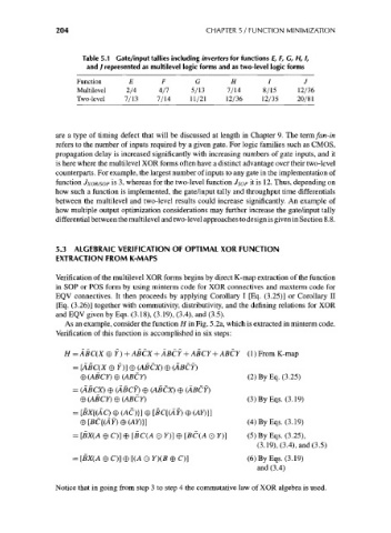
Table 5.1 Gate/input tallies including inverters for functions E, F, G, H, I,
and / represented as multilevel logic forms and as two-level logic forms
Function E F G H I J
Multilevel 2/4 4/7 5/13 7/14 8/15 12/36
Two-level 7/13 7/14 11/21 12/36 12/35 20/81

are a type of timing defect that will be discussed at length in Chapter 9. The term fan-in
refers to the number of inputs required by a given gate. For logic families such as CMOS,
propagation delay is increased significantly with increasing numbers of gate inputs, and it
is here where the multilevel XOR forms often have a distinct advantage over their two-level
counterparts. For example, the largest number of inputs to any gate in the implementation of
function JXOR/SOP is 3, whereas for the two-level function JSOP it is 12. Thus, depending on
how such a function is implemented, the gate/input tally and throughput time differentials
between the multilevel and two-level results could increase significantly. An example of
how multiple output optimization considerations may further increase the gate/input tally
differential between the multilevel and two-level approaches to design is given in Section 8.8.

5.3 ALGEBRAIC VERIFICATION OF OPTIMAL XOR FUNCTION
EXTRACTION FROM K-MAPS

Verification of the multilevel XOR forms begins by direct K-map extraction of the function
in SOP or POS form by using minterm code for XOR connectives and maxterm code for
EQV connectives. It then proceeds by applying Corollary I [Eq. (3.25)] or Corollary II
[Eq. (3.26)] together with commutivity, distributivity, and the defining relations for XOR
and EQV given by Eqs. (3.18), (3.19), (3.4), and (3.5).
As an example, consider the function H in Fig. 5.2a, which is extracted in minterm code.
Verification of this function is accomplished in six steps:

H = ABC(X ® Y) + ABCX + ABCY + ABCY + ABCY (1) From K-map
= [ABC(X 0 7)] 0 (ABCX) 0 (ABCY)
0 (ABCY) 0 (ABCY) (2) By Eq. (3.25)
= (ABCX) 0 (ABCY) 0 (ABCX) 0 (ABCY)
0 (ABCY) 0 (ABCY) (3) By Eqs. (3.19)
= [BX{(AQ 0 (AC)}] 0 [BC{(AY) 0 (AY)}]
®[BC{(AY)@(AY)}] (4) By Eqs. (3.19)
= [BX(A 0 C)] 0 [BC(A O F)] 0 [BC(A O Y)] (5) By Eqs. (3.25),
(3.19), (3.4), and (3.5)

= [BX(A 0 C)] 0 [(A O Y)(B 0 C)] (6) By Eqs. (3.19)
and (3.4)

Notice that in going from step 3 to step 4 the commutative law of XOR algebra is used.