Page 151 - Engineering Electromagnetics, 8th Edition

CHAPTER 5 Conductors and Dielectrics 133

As soon as we establish a value for any of these three fields within the dielectric, the
other two can be found immediately. The difficulty lies in crossing over the boundary
from the known fields external to the dielectric to the unknown ones within it. To do
this we need a boundary condition, and this is the subject of the next section. We will
complete this example then.
In the remainder of this text we will describe polarizable materials in terms of D
and rather than P and χ e .We will limit our discussion to isotropic materials.

D5.8. A slab of dielectric material has a relative dielectric constant of 3.8 and
2
contains a uniform electric flux density of 8 nC/m .If the material is lossless,
find: (a) E;(b) P;(c) the average number of dipoles per cubic meter if the
average dipole moment is 10 −29 C · m.
2
Ans. 238 V/m; 5.89 nC/m ;5.89 × 10 20 m −3

5.8 BOUNDARY CONDITIONS FOR PERFECT
DIELECTRIC MATERIALS
How do we attack a problem in which there are two different dielectrics, or a dielectric
and a conductor? This is another example of a boundary condition, such as the condi-
tion at the surface of a conductor whereby the tangential fields are zero and the normal
electric flux density is equal to the surface charge density on the conductor. Now we
take the first step in solving a two-dielectric problem, or a dielectric-conductor prob-
lem, by determining the behavior of the fields at the dielectric interface.
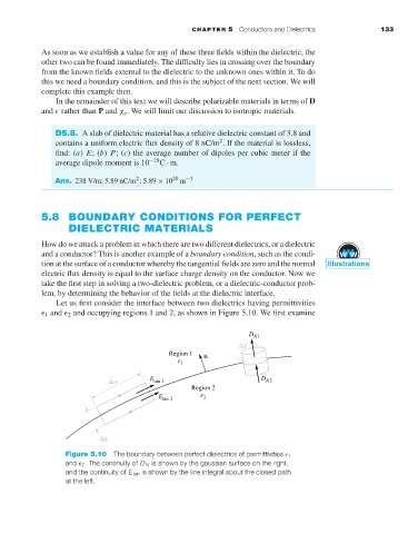
Let us first consider the interface between two dielectrics having permittivities
1 and 2 and occupying regions 1 and 2, as shown in Figure 5.10. We first examine

n

Figure 5.10 The boundary between perfect dielectrics of permittivities 1
and 2 . The continuity of D N is shown by the gaussian surface on the right,
and the continuity of E tan is shown by the line integral about the closed path
at the left.