Page 233 - Engineering Electromagnetics, 8th Edition

CHAPTER 7 The Steady Magnetic Field 215

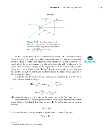
Figure 7.19 The differential current
element Idza z at the origin establishes the
differential vector magnetic potential field,
µ 0 Idza z
dA = at P(ρ, φ, z).
4π ρ + z 2
2
We note that the direction of dA is the same as that of IdL. Each small section
of a current-carrying conductor produces a contribution to the total vector magnetic
potential which is in the same direction as the current flow in the conductor. The
magnitude of the vector magnetic potential varies inversely with the distance to the
current element, being strongest in the neighborhood of the current and gradually
10
falling off to zero at distant points. Skilling describes the vector magnetic potential
field as “like the current distribution but fuzzy around the edges, or like a picture of
the current out of focus.”
In order to find the magnetic field intensity, we must take the curl of (49) in
cylindrical coordinates, leading to
1 1 ∂dA z
dH = ∇× dA = − a φ
µ 0 µ 0 ∂ρ
or
Idz ρ
dH = a φ
4π (ρ + z )
2 3/2
2
which is easily shown to be the same as the value given by the Biot-Savart law.
Expressions for the vector magnetic potential A can also be obtained for a current
source which is distributed. For a current sheet K, the differential current element
becomes
IdL = K dS

In the case of current flow throughout a volume with a density J,wehave
IdL = J dν

10 See the References at the end of the chapter.