Page 229 - Engineering Electromagnetics, 8th Edition

CHAPTER 7 The Steady Magnetic Field 211

or
2
∇ V m = 0(J = 0) (44)

We will see later that V m continues to satisfy Laplace’s equation in homogeneous
magnetic materials; it is not defined in any region in which current density is present.
Although we shall consider the scalar magnetic potential to a much greater extent
in Chapter 8, when we introduce magnetic materials and discuss the magnetic circuit,
one difference between V and V m should be pointed out now: V m is not a single-valued
function of position. The electric potential V is single-valued; once a zero reference is
assigned, there is only one value of V associated with each point in space. Such is not
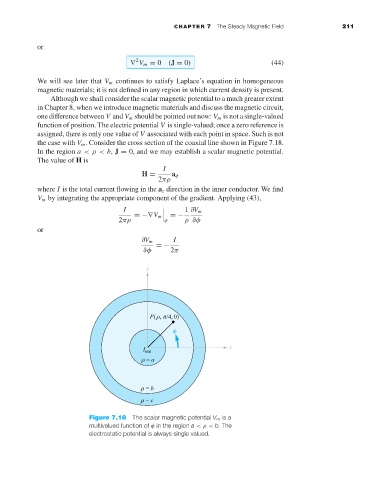
the case with V m . Consider the cross section of the coaxial line shown in Figure 7.18.
In the region a <ρ < b, J = 0, and we may establish a scalar magnetic potential.
The value of H is
I
H = a φ
2πρ
where I is the total current flowing in the a z direction in the inner conductor. We find
V m by integrating the appropriate component of the gradient. Applying (43),
I 1 ∂V m

=−∇V m =−
2πρ φ ρ ∂φ
or
∂V m I
=−
∂φ 2π

Figure 7.18 The scalar magnetic potential V m is a
multivalued function of φ in the region a <ρ < b. The
electrostatic potential is always single valued.