Page 276 - Engineering Electromagnetics, 8th Edition

258 ENGINEERING ELECTROMAGNETICS

and obtain

NI 500 × 4
H φ = = = 2120 A/m
2πr 6.28 × 0.15
at the mean radius.
Our magnetic circuit in this example does not give us any opportunity to find the
mmf across different elements in the circuit, for there is only one type of material.
The analogous electric circuit is, of course, a single source and a single resistor. We
could make it look just as long as the preceding analysis, however, if we found the
current density, the electric field intensity, the total current, the resistance, and the
source voltage.
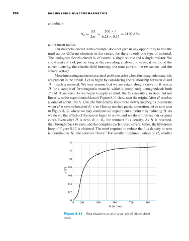
More interesting and more practical problems arise when ferromagnetic materials
are present in the circuit. Let us begin by considering the relationship between B and
H in such a material. We may assume that we are establishing a curve of B versus
H for a sample of ferromagnetic material which is completely demagnetized; both
B and H are zero. As we begin to apply an mmf, the flux density also rises, but not
linearly, as the experimental data of Figure 8.11 show near the origin. After H reaches
avalue of about 100 A · t/m, the flux density rises more slowly and begins to saturate
when H is several hundred A · t/m. Having reached partial saturation, let us now turn
to Figure 8.12, where we may continue our experiment at point x by reducing H.As
we do so, the effects of hysteresis begin to show, and we do not retrace our original
curve. Even after H is zero, B = B r , the remnant flux density. As H is reversed,
then brought back to zero, and the complete cycle traced several times, the hysteresis
loop of Figure 8.12 is obtained. The mmf required to reduce the flux density to zero
is identified as H c , the coercive “force.” For smaller maximum values of H, smaller

Figure 8.11 Magnetization curve of a sample of silicon sheet
steel.