Page 574 - Engineering Electromagnetics, 8th Edition

556 ENGINEERING ELECTROMAGNETICS

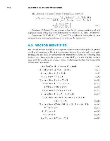
The Laplacian of a scalar is found by using (A.2) and (A.3):
1 ∂ h 2 h 3 ∂ν ∂ h 3 h 1 ∂V
2
∇ V =∇ · ∇V = +
h 1 h 2 h 3 ∂u h 1 ∂u ∂ν h 2 ∂ν
∂ h 1 h 2 ∂V
+ (A.5)
∂w h 3 ∂w
Equations (A.2) to (A.5) may be used to find the divergence, gradient, curl, and
Laplacian in any orthogonal coordinate system for which h 1 , h 2 , and h 3 are known.
2
Expressions for ∇ · D, ∇V , ∇× H, and ∇ V are given in rectangular, circular
cylindrical, and spherical coordinate systems inside the back cover.

A.3 VECTOR IDENTITIES

The vector identities that follow may be proved by expansion in rectangular (or general
curvilinear) coordinates. The first two identities involve the scalar and vector triple
products, the next three are concerned with operations on sums, the following three
apply to operations when the argument is multiplied by a scalar function, the next
three apply to operations on scalar or vector products, and the last four concern the
second-order operations.
(A × B) · C ≡ (B × C) · A ≡ (C × A) · B (A.6)
A × (B × C) ≡ (A · C)B − (A · B)C (A.7)
∇ · (A + B) ≡∇ · A +∇ · B (A.8)
∇(V + W) ≡∇V +∇W (A.9)
∇× (A + B) ≡∇ × A +∇ × B (A.10)
∇ · (V A) ≡ A · ∇V + V ∇ · A (A.11)
∇(VW) ≡ V ∇W + W∇V (A.12)
∇× (V A) ≡∇V × A + V ∇× A (A.13)
∇ · (A × B) ≡ B · ∇× A − A · ∇× B (A.14)
∇(A · B) ≡ (A · ∇)B + (B · ∇)A + A × (∇× B)
+ B × (∇× A) (A.15)
∇× (A × B) ≡ A∇ · B − B∇ · A + (B · ∇)A − (A · ∇)B (A.16)
2
∇· ∇V ≡∇ V (A.17)
∇· ∇× A ≡ 0 (A.18)
∇× ∇V ≡ 0 (A.19)
2
∇× ∇× A ≡∇(∇ · A) −∇ A (A.20)