Page 72 - Essentials of physical chemistry

34 Essentials of Physical Chemistry

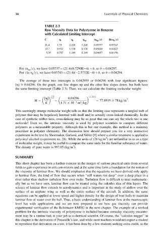
TABLE 2.3
Raw Viscosity Data for Polystyrene in Benzene
with Calculated Limiting Intercept
C h h r h sp (h sp =c) (ln h r =c)
21.4 1.35 2.228 1.228 0.05737 0.03743
10.7 0.932 1.538 0.538 0.05028 0.04023
5.35 0.757 1.249 0.249 0.04657 0.04156

For (h =c), we have 0.05737 ¼ (21.4)(6.7290E 4) þ b,so b ¼ 0.04297.
sp
For (ln h =c), we have 0.03743 ¼ (21.4)( 2.5732E 4) þ b,so b ¼ 0.04294.
r
The average of these two intercepts is 0.042955 or 0.04296 with four significant figures:
[h] ffi 0:04296. On the graph, one line slopes up and the other line slopes down, but both have
the same limiting intercept (Table 2.3). Then, we can calculate the limiting molecular weight:

1
(1:351)
[h] a ðÞ 0:04296 3
¼ 77:8919 ffi 78 kg=m :
M ¼ ¼ 3 3
K 1:71 10 m =kg
This seemingly strange molecular weight tells us that the limiting case represents a tangled web of
polymer that may be hopelessly knotted with itself and=or actually cross-linked chemically. In the
case of synthetic rubber tires, cross-linking may be so great that one can say the whole tire is one
molecule! Even so, the intrinsic viscosity is used by polymer scientists to compare different
polymers as a measurable property. Although this is but one example, this method is a mainstay
procedure in polymer chemistry. The discussion here should prepare you for a very instructive
experiment in the text by Shoemaker, Garland, and Nibler [9] where a similar treatment is applied to
3
polyvinyl alcohol (experiment no. 28). While the units of (78 kg=m ) are unfamiliar to us as a type
of molecular weight, it may be useful to compare the same units for the familiar substance of water.
3
The density of pure water is 997.05 (kg=m ).

SUMMARY
This short chapter has been a further exercise in the merger of various practical units from several
fields to gain experience in unit conversions and at the same time form a foundation for the notion of
the viscosity of laminar flow. We should emphasize that the equations we have derived only apply
to laminar flow, the kind of flow that occurs when ‘‘still waters run deep’’ over a deep place in a
river rather than shallow turbulent flow over rocks. Turbulent flow is difficult to treat mathematic-
ally but as we have seen, laminar flow can be treated using the calculus idea of thin layers. The
science of laminar flow extends to aerodynamics and is important in the study of airflow over the
surface of an airplane wing as well as the entire surface of the aircraft. In addition, the same
equations can be applied at lower speed and higher density for the design of boat hulls to maintain
laminar flow of water over the hull. Thus, a basic understanding of laminar flow at the macroscopic
level has wide applications and we are now prepared to see how gas viscosity can provide
experimental verification of the Boltzmann KMTG in the next chapter. The example of a worked
problem for the intrinsic viscosity of polystyrene is included because someday viscosity measure-
ment may be a routine task in your job as a chemical scientist. Of course, the ‘‘calculus nugget’’ in
this chapter is the derivation of Poiseuille’s law, and while most teachers would not expect a student
to reproduce that derivation on a test, it has been done by a few students seeking extra credit, so the