Page 245 - Excel 2007 Bible

16_044039 ch11.qxp 11/21/06 11:04 AM Page 202
Part II
Working with Formulas and Functions
FIGURE 11.18
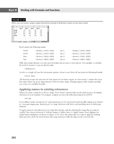
When you use names, using a range-intersection formula to determine values is even more useful.
Excel created the following names:
North
Qtr1
=Sheet1!$B$2:$E$2
=Sheet1!$B$2:$B$5
South
=Sheet1!$B$3:$E$3
=Sheet1!$C$2:$C$5
Qtr2
West
Qtr3
=Sheet1!$B$4:$E$4
=Sheet1!$D$2:$D$5
East
Qtr4
=Sheet1!$E$2:$E$5
=Sheet1!$B$5:$E$5
With these names defined, you can create formulas that are easy to read and use. For example, to calculate
the total for Quarter 4, just use this formula:
=SUM(Qtr4)
To refer to a single cell, use the intersection operator. Move to any blank cell and enter the following formula:
=Qtr1 West
This formula returns the value for the first quarter for the West region. In other words, it returns the value
that exists where the Qtr1 range intersects with the West range. Naming ranges in this manner can help
you create very readable formulas.
Applying names to existing references
When you create a name for a cell or a range, Excel doesn’t automatically use the name in place of existing
references in your formulas. For example, suppose you have the following formula in cell F10:
=A1–A2
If you define a name Income for A1 and Expenses for A2, Excel won’t automatically change your formula
to =Income–Expenses. Replacing cell or range references with their corresponding names is fairly easy,
however.
To apply names to cell references in formulas after the fact, start by selecting the range that you want to
modify. Then choose Formulas ➪ Defined Names ➪ Define Name ➪ Apply Names. Excel displays the
Apply Names dialog box, as shown in Figure 11.19. Select the names that you want to apply by clicking
them and then click OK. Excel replaces the range references with the names in the selected cells.

202