Page 256 - Excel 2007 Bible

17_044039 ch12.qxp 11/21/06 11:05 AM Page 213
The formulas in column D graphically depict the sales numbers in column B by displaying a series of char-
acters in the Wingdings font. This example uses character code 61 (an equal sign), which appears on-screen
as a small floppy disc the Wingdings font. A formula using the REPT function determines the number of
characters displayed. The formula in cell D2 is:
=REPT(“=”,B2/100)
Assign the Wingdings font to cells D2, and then copy the formulas down the column to accommodate all
the data. Depending on the numerical range of your data, you may need to change the scaling. Experiment
by replacing the 100 value in the formulas. You can substitute any character you like for the equal sign
character in the formula to produce a different character in the chart.
The workbook shown in Figure 12.3 also appears on the companion CD-ROM. The file is
ON the CD-ROM
ON the CD-ROM
named text histogram.xlsx.
Padding a number
You’re probably familiar with a common security measure (frequently used on printed checks) in which
numbers are padded with asterisks on the right. The following formula displays the value in cell A1, along
with enough asterisks to make a total of 24 characters:
=(A1 & REPT(“*”,24-LEN(A1))) Creating Formulas That Manipulate Text 12
If you’d prefer to pad the number with asterisks on the left instead, use this formula:
=REPT(“*”,24-LEN(A1))&A1
The formula below displays 12 asterisks on both sides of the number.
=REPT(“*”,12)&A1&REPT(“*”,12)
The preceding formulas are a bit deficient because they don’t show any number formatting. This revised
version displays the value in A1 (formatted), along with the asterisk padding on the right:
=(TEXT(A1,”$#,##0.00”)&REPT(“*”,24-LEN(TEXT(A1,”$#,##0.00”))))
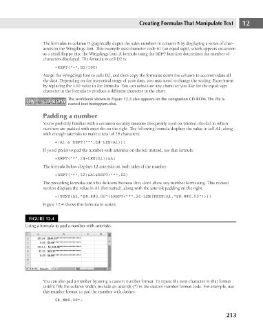
Figure 12.4 shows this formula in action.
FIGURE 12.4
Using a formula to pad a number with asterisks.

You can also pad a number by using a custom number format. To repeat the next character in that format
until it fills the column width, include an asterisk (*) in the custom number format code. For example, use
this number format to pad the number with dashes:
$#,##0.00*-

213