Page 146 - Excel Workbook for Dummies

14_798452 ch09.qxp 3/13/06 7:52 PM Page 129
Chapter 9: Using Math Functions 129
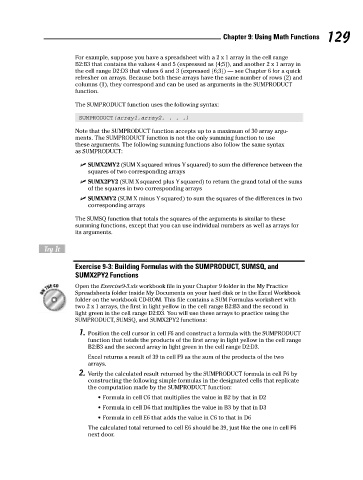
For example, suppose you have a spreadsheet with a 2 x 1 array in the cell range
B2:B3 that contains the values 4 and 5 (expressed as {4;5}), and another 2 x 1 array in
the cell range D2:D3 that values 6 and 3 (expressed {6;3}) — see Chapter 6 for a quick
refresher on arrays. Because both these arrays have the same number of rows (2) and
columns (1), they correspond and can be used as arguments in the SUMPRODUCT
function.

The SUMPRODUCT function uses the following syntax:

SUMPRODUCT(array1,array2, . . .)

Note that the SUMPRODUCT function accepts up to a maximum of 30 array argu-
ments. The SUMPRODUCT function is not the only summing function to use
these arguments. The following summing functions also follow the same syntax
as SUMPRODUCT:
SUMX2MY2 (SUM X squared minus Y squared) to sum the difference between the
squares of two corresponding arrays
SUMX2PY2 (SUM X squared plus Y squared) to return the grand total of the sums
of the squares in two corresponding arrays
SUMXMY2 (SUM X minus Y squared) to sum the squares of the differences in two
corresponding arrays
The SUMSQ function that totals the squares of the arguments is similar to these
summing functions, except that you can use individual numbers as well as arrays for
its arguments.

Try It

Exercise 9-3: Building Formulas with the SUMPRODUCT, SUMSQ, and
SUMX2PY2 Functions
Open the Exercise9-3.xls workbook file in your Chapter 9 folder in the My Practice
Spreadsheets folder inside My Documents on your hard disk or in the Excel Workbook
folder on the workbook CD-ROM. This file contains a SUM Formulas worksheet with
two 2 x 1 arrays, the first in light yellow in the cell range B2:B3 and the second in
light green in the cell range D2:D3. You will use these arrays to practice using the
SUMPRODUCT, SUMSQ, and SUMX2PY2 functions:

1. Position the cell cursor in cell F6 and construct a formula with the SUMPRODUCT
function that totals the products of the first array in light yellow in the cell range
B2:B3 and the second array in light green in the cell range D2:D3.
Excel returns a result of 39 in cell F9 as the sum of the products of the two
arrays.
2. Verify the calculated result returned by the SUMPRODUCT formula in cell F6 by
constructing the following simple formulas in the designated cells that replicate
the computation made by the SUMPRODUCT function:
• Formula in cell C6 that multiplies the value in B2 by that in D2
• Formula in cell D6 that multiplies the value in B3 by that in D3
• Formula in cell E6 that adds the value in C6 to that in D6
The calculated total returned to cell E6 should be 39, just like the one in cell F6
next door.