Page 172 - Excel for Scientists and Engineers: Numerical Methods

CHAPTER 8 ROOTS OF EOUATIONS 149

Once a chart has been created, it is very easy to expand the scales of the axes
to examine the crossing region at higher and higher magnification. Figure 8-3
shows part of the data table used to create Figure 8-2; the formula in column B is
the function shown in equation 8-1. The two values that bracket one of the roots
of the function are highlighted.

0.0004

0.0003
0.0002

0.0001

0

-0.0001

-0.0002

-0.0003

-0.0004
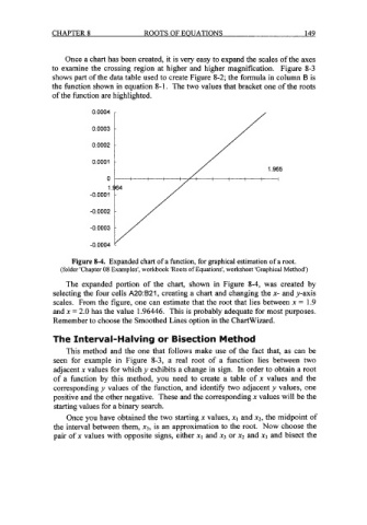
Figure 8-4. Expanded chart of a function, for graphical estimation of a root.
(folder 'Chapter 08 Examples', workbook 'Roots of Equations', worksheet 'Graphical Method')
The expanded portion of the chart, shown in Figure 8-4, was created by
selecting the four cells A20:B21, creating a chart and changing the x- and y-axis
scales. From the figure, one can estimate that the root that lies between x = 1.9
and x = 2.0 has the value 1.96446. This is probably adequate for most purposes.
Remember to choose the Smoothed Lines option in the Chartwizard.

The Interval-Halving or Bisection Method
This method and the one that follows make use of the fact that, as can be
seen for example in Figure 8-3, a real root of a function lies between two
adjacent x values for which y exhibits a change in sign. In order to obtain a root
of a function by this method, you need to create a table of x values and the
corresponding y values of the function, and identify two adjacent y values, one
positive and the other negative. These and the corresponding x values will be the
starting values for a binary search.
Once you have obtained the two starting x values, xI and x2, the midpoint of
the interval between them, x3, is an approximation to the root. Now choose the
pair of x values with opposite signs, either x1 and x3 or x2 and x3 and bisect the