Page 223 - Excel for Scientists and Engineers: Numerical Methods

200 EXCEL: NUMERICAL METHODS

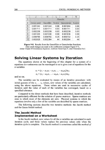
Figure 9-8. Results from the GaussElim or GaussJordan functions
when small changes are made in the coefficients (compare Figure 9-7),
(folder 'Chapter 09 Simultaneous Equations', workbook 'Simult Eqns 11', sheet 'Elimination Fns')

Solving Linear Systems by Iteration
The equations shown at the beginning of this chapter for a system of n
equations in n unknowns can be rearranged so as to give a set of equations for the
n variables
x1 = (c1 - al2x2 - a13x3 . . . - al&n)/all
x2 = (c2 - a23x3 . . .- a21& - a21Xl)/a22
and so on.
The variables can be evaluated by means of an iterative procedure: with
initial guesses of the xl . . . x, values, new values of the variables are calculated,
using the above equations. These values are used in successive cycles of
iteration until the value of each of the variables has converged, based on a
specified tolerance.
Compared to the direct methods that have been described, iterative methods
are particularly efficient for the solution of sparse matrices. Sparse matrices are
ones in which most of the elements are zero. Physical systems in which the
equations involve only a few of the variables are described by sparse matrices.
The following sections describe two iterative methods: the Jacobi method
and the Gauss-Seidel method.

The Jacobi Method
Implemented on a Worksheet

In the Jacobi method, new values for all the n variables are calculated in each
iteration cycle, and these values replace the previous values only when the
iteration cycle is complete. The Jacobi method is sometimes called the method of