Page 281 - Excel for Scientists and Engineers: Numerical Methods

258 EXCEL: NUMERICAL METHODS

Solving a Second-Order Ordinary Differential Equation
by the Finite-Difference Method:
Another Example
In preceding sections, we used Euler's method and the Runge-Kutta method
to solve the second-order differential equation y" - y = 0 by the shooting method.
This differential equation can be solved readily by using the finite-difference
method.
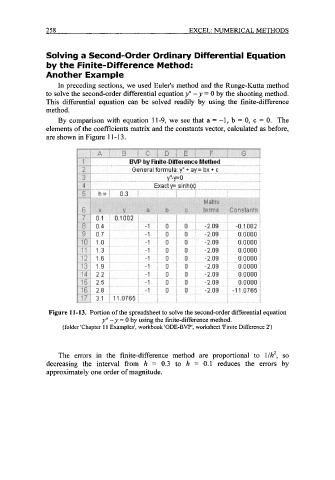
By comparison with equation 11-9, we see that a = -1, b = 0, c = 0. The
elements of the coefficients matrix and the constants vector, calculated as before,
are shown in Figure 1 1 - 13.

Figure 11-13. Portion of the spreadsheet to solve the second-order differential equation
y" - y = 0 by using the finite-difference method.
(folder 'Chapter 1 1 Examples', workbook 'ODE-BVP', worksheet 'Finite Difference 2')

The errors in the finite-difference method are proportional to llh2, so
decreasing the interval from h = 0.3 to h = 0.1 reduces the errors by
approximately one order of magnitude.