Page 278 - Excel for Scientists and Engineers: Numerical Methods

CHAPTER 11 ORDINARY DIFFERENTIAL EQUATIONS. PART I1 255

for each subinterval. Since y is known at the ends of the interval, we need to
write only nine simultaneous equations (e.g., at x2 = 1.2):
y~ i- ((0.2)2(- 0.15 + x2/2.3) - 2)y2 +y3 = (0.2)2~2 (1 1-15)
2 - 1.985~2 + J+ = 0.048 (11-15a)

1 .985y2 + y3 = -1.952 (1 1-15b)

at x3 = 1.4:
y2 - (2 - (0.15 - ~3/2.3)(0.2)~)~, = (0.2)2~3 (1 1-16)
+y4
y2 - 1.982~3 + y4 = 0.056 (1 1 - 16a)
and at xIo = 2.8:
y9-(2 -(0.15 -xl0/2.3)(0.2)~)ylo +yll=(0.2)2~10 (1 1-17)
y9- 1.957ylo- 1 =0.112 (1 1-17a)

y9- 1.957ylo= 1.112 (1 1-17b)
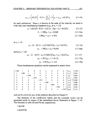
These simultaneous equations can be expressed in matrix form:

-1.985 I 0 0 0 0 0 0 0 -1.952
1 -1.982 1 0 0 0 0 0 0 0.056
0 1 -1.978 1 0 0 0 0 0 0.064
0 0 1 -1.975 1 0 0 0 0 0.072
0 0 0 1 -1.971 1 0 0 0 0.080
0 0 0 0 1 -1.968 1 0 0 0.088
0 0 0 0 0 1 - -1.964 1 0 0.096
0 0 0 0 0 0 1 -1.961 1 0.104
0 0 0 0 0 0 0 1 -1.957 1.1 12

and can be solved by any of the methods described in Chapter 9.
The elements of the coefficients matrix and the constants vector can be
generated easily by means of the spreadsheet layout illustrated in Figure 11-10.
The formulas in cells C9 and F9 are, respectively,

=-(p-dq)
=-( 2-a*h A2)