Page 274 - Excel for Scientists and Engineers: Numerical Methods

CHAPTER 11 ORDINARY DIFFERENTIAL EQUATIONS. PART I1 25 1

The Eulerk method calculation was performed in two steps in these two cells
so as to make it convenient to convert to the RK calculation, as will be described
in the following section.
Using an initial estimate of 1 for dy/dx, the boundary value at x = 2.0, in cell
F34, is 3.3030. Goal Seek was used to find the value of z that produced the
desired boundary value, y = 3.63. The final calculations are shown in Figure 1 1 -
7, together with the values calculated from the exact expression, y = sinh x, and
the percentage error.

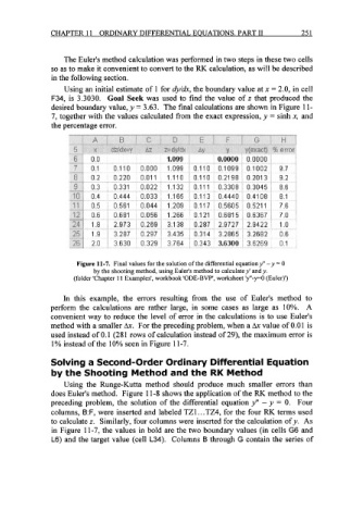
Figure 11-7. Final values for the solution of the differential equation y" -y = 0
by the shooting method, using Euler's method to calculate y' and y.
(folder 'Chapter 1 1 Examples', workbook 'ODE-BVP', worksheet 'y"-y'O (Euler)')

In this example, the errors resulting from the use of Eulerls method to
perform the calculations are rather large, in some cases as large as 10%. A
convenient way to reduce the level of error in the calculations is to use Euler's
method with a smaller hx. For the preceding problem, when a hx value of 0.01 is
used instead of 0.1 (281 rows of calculation instead of 29), the maximum error is
1% instead of the 10% seen in Figure 11-7.

Solving a Second-Order Ordinary Differential Equation
by the Shooting Method and the RK Method

Using the Runge-Kutta method should produce much smaller errors than
does Euler's method. Figure 11-8 shows the application of the RK method to the
preceding problem, the solution of the differential equation y" - y = 0. Four
columns, B:F, were inserted and labeled TZ1.. .TZ4, for the four RK terms used
to calculate z. Similarly, four columns were inserted for the calculation of y. As
in Figure 11-7, the values in bold are the two boundary values (in cells G6 and
L6) and the target value (cell L34). Columns B through G contain the series of