Page 272 - Excel for Scientists and Engineers: Numerical Methods

CHAPTER 11 ORDINARY DIFFERENTIAL EOUATIONS. PART I1 249

The calculated value of z for the required boundary value is shown in the
third row of the table. The formula in cell H8 is
=H6-16*(H7-H6)/(17-16)

If the problem is linear, the interpolated value of z obtained in this way will
be the desired solution. The spreadsheet with final values is shown in Figure 11-
4. A similar spreadsheet in which the y values were calculated using the Runge
custom function can be seen on the CD-ROM.
This "shooting" procedure was performed manually-that is, successive trial
values were entered into the spreadsheet, and the resulting values copied and
pasted into the cells shown in Figure 1 1-3, in order to use interpolation to find the
final value. You can obtain the same final result essentially in one step by using
Goal Seek. After entering a trial value, z = 0, in cell C6, use Goal Seek to change
cell C6 to make the target cell, 61 85, attain a value of zero.
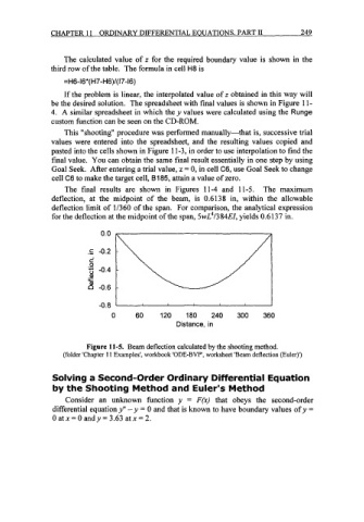
The final results are shown in Figures 11-4 and 11-5. The maximum
deflection, at the midpoint of the beam, is 0.6138 in, within the allowable
deflection limit of 1/360 of the span. For comparison, the analytical expression
for the deflection at the midpoint of the span, 5wL4/384EI, yields 0.6137 in.

0 60 120 180 240 300 360
Distance, in

Figure 11-5. Beam deflection calculated by the shooting method.
(folder 'Chapter I 1 Examples', workbook 'ODE-BVP', worksheet 'Beam deflection (Euler)')

Solving a Second-Order Ordinary Differential Equation
by the Shooting Method and Euler's Method
Consider an unknown function y = F(x) that obeys the second-order
differential equation y" - y = 0 and that is known to have boundary values of y =
0 atx= 0 and y = 3.63 atx = 2.