Page 271 - Excel for Scientists and Engineers: Numerical Methods

248 EXCEL: NUMERICAL METHODS

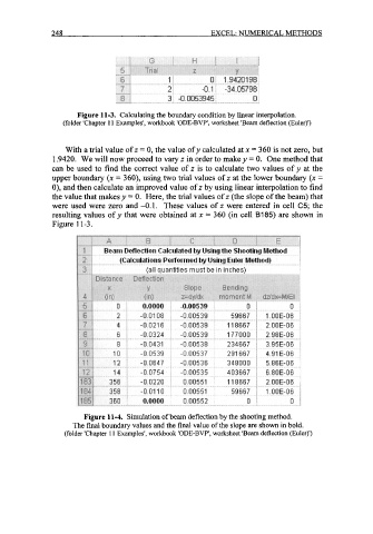
Figure 11-3. Calculating the boundary condition by linear interpolation.
(folder 'Chapter 1 1 Examples', workbook 'ODE-BVP', worksheet 'Beam deflection (Euler)')

With a trial value of z = 0, the value of y calculated at x = 360 is not zero, but
1.9420. We will now proceed to vary z in order to make y = 0. One method that
can be used to find the correct value of z is to calculate two values of y at the
upper boundary (x = 360), using two trial values of z at the lower boundary (x =
0), and then calculate an improved value of z by using linear interpolation to find
the value that makes y = 0. Here, the trial values of z (the slope of the beam) that
were used were zero and -0.1. These values of z were entered in cell C5; the
resulting values of y that were obtained at x = 360 (in cell B185) are shown in
Figure 11-3.

Figure 11-4. Simulation of beam deflection by the shooting method.
The final boundary values and the final value of the slope are shown in bold.
(folder 'Chapter 1 1 Examples', workbook 'ODE-BVP', worksheet 'Beam deflection (Euler)')