Page 209 - Fiber Bragg Gratings

186 Chapter 4 Theory of Fiber Bragg Gratings

model the refractive index profile of the grating, the period may be subdi-
vided into further sections. A recursive technique is then applied to calcu-
late the reflectivity of the composite period of the grating. Thus, the
problem is reduced to calculating the amplitude reflectivity p of each
single period. The processes is repeated for N single-period sections, each
with any local function for the refractive index modulation, period, or
phase steps. It is easy to realize that any type of grating, microns or
meters long, is then easily modeled. Alternatively, for certain types of
pure sinusoidal refractive index modulation, the analytical solution for
the constant period grating can be used [Eq. (4.3.11)] so long as the
conditions described in Section 4.8.2 are adhered to. The power of this
technique is, however, restricted by the computational errors when calcu-
lating the reflectivity and transmission of a large number of thin films.
Despite this restriction, many types of gratings are adequately realized,
provided the maximum reflectivity is limited to values ~99.99%. With
care and appropriate computational algorithms, better results may be
possible. The basic analysis is similar to the T-matrix approach; however,
the reflectivity is simply calculated from the difference in the refractive
index between two adjacent layers.

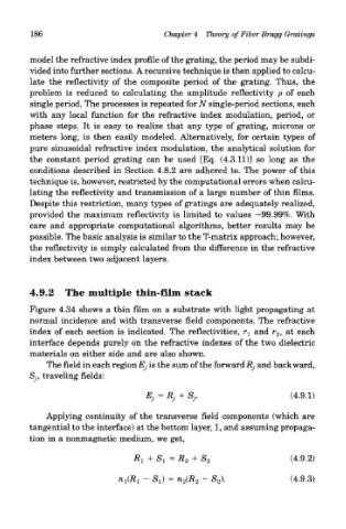
4.9.2 The multiple thin-film stack
Figure 4.34 shows a thin film on a substrate with light propagating at
normal incidence and with transverse field components. The refractive
index of each section is indicated. The reflectivities, r x and r 2, at each
interface depends purely on the refractive indexes of the two dielectric
materials on either side and are also shown.
The field in each region Ej is the sum of the forward Rj and backward,
Sj, traveling fields:

Applying continuity of the transverse field components (which are
tangential to the interface) at the bottom layer, 1, and assuming propaga-
tion in a nonmagnetic medium, we get,