Page 286 - Fluid-Structure Interactions Slender Structure and Axial Flow (Volume 1)

PIPES CONVEYING FLUID: LINEAR DYNAMICS I1 267

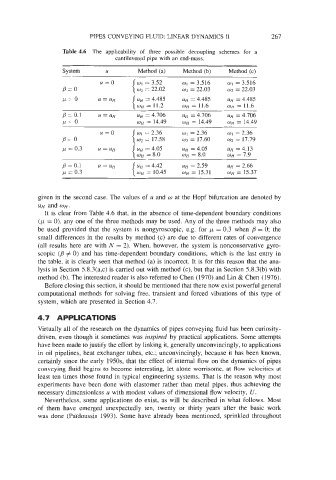
Table 4.6 The applicability of three possible decoupling schemes for a
cantilevered pipe with an end-mass.

System U Method (a) Method (b) Method (c)
WI = 3.516 ~1 = 3.516
W? = 22.03 ~2 = 22.03
UH = 4.485 UH = 4.485
WH = 11.6 WH = 11.6
UH = 4.706 UH = 4.706
WH = 14.49 WH = 14.49
~1 = 2.36 WI = 2.36
W? = 17.60 ~2 = 17.79
UH = 4.05 UH = 4.13
WH = 8.0 WH = 7.9

given in the second case. The values of u and w at the Hopf bifurcation are denoted by
UH and WH.
It is clear from Table 4.6 that, in the absence of time-dependent boundary conditions
(p = 0), any one of the three methods may be used. Any of the three methods may also
be used provided that the system is nongyroscopic, e.g. for p = 0.3 when /3 = 0; the
small differences in the results by method (c) are due to different rates of convergence
(all results here are with N = 2). When, however, the system is nonconservative gyro-
scopic (B # 0) and has time-dependent boundary conditions, which is the last entry in
the table, it is clearly seen that method (a) is incorrect. It is for this reason that the ana-
lysis in Section 5.8.3(a,c) is carried out with method (c), but that in Section 5.8.3(b) with
method (b). The interested reader is also referred to Chen (1970) and Lin & Chen (1976).
Before closing this section, it should be mentioned that there now exist powerful general
computational methods for solving free, transient and forced vibrations of this type of
system, which are presented in Section 4.7.

4.7 APPLICATIONS
Virtually all of the research on the dynamics of pipes conveying fluid has been curiosity-
driven, even though it sometimes was inspired by practical applications. Some attempts
have been made to justify the effort by linking it, generally unconvincingly, to applications
in oil pipelines, heat exchanger tubes, etc.; unconvincingly, because it has been known,
certainly since the early 1950s, that the effect of internal flow on the dynamics of pipes
conveying fluid begins to become interesting, let alone worrisome, at flow vclocities at
least ten times those found in typical engineering systems. That is the reason why most
experiments have been done with elastomer rather than metal pipes, thus achieving the
necessary dimensionless u with modest values of dimensional flow velocity, U.
Nevertheless, some applications do exist, as will be described in what follows. Most
of them have emerged unexpectedly ten, twenty or thirty years after the basic work
was done (Paldoussis 1993). Some have already been mentioned, sprinkled throughout