Page 119 - Formation Damage during Improved Oil Recovery Fundamentals and Applications

Formation Damage by Fines Migration: Mathematical and Laboratory Modeling, Field Cases 101

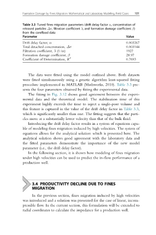
Table 3.3 Tuned fines-migration parameters (drift delay factor α, concentration of
released particles Δσ, filtration coefficient λ, and formation damage coefficient β)
from the coreflood data
Parameter Value
Drift delay factor, α 0.003267
Total detached concentration, Δσ 0.003144
Filtration coefficient, λ (1/m) 1927
Formation damage coefficient, β 28.97
Coefficient of Determination, R 2 0.7693

The data were fitted using the model outlined above. Both datasets
were fitted simultaneously using a genetic algorithm least-squared fitting
procedure implemented in MATLAB (Mathworks, 2010). Table 3.3 pre-
sents the four parameters obtained by fitting the experimental data.
The fitting in Fig. 3.12 shows good agreement between the experi-
mental data and the theoretical model. The stabilization time of this
experiment highly exceeds the time to inject a single-pore volume and
this feature is captured in the value of the drift delay factor in Table 3.3,
which is significantly smaller than one. The fitting suggests that the parti-
cles move at a substantially lower velocity than that of the bulk fluid.
Introducing the drift delay factor results in a system of equations capa-
ble of modeling fines migration induced by high velocities. The system of
equations allows for the analytical solution which is presented here. The
analytical solution shows good agreement with the laboratory data and
the fitted parameters demonstrate the importance of the new model
parameter (i.e., the drift delay factor).
In the following section, it is shown how modeling of fines migration
under high velocities can be used to predict the in-flow performance of a
production well.

3.4 PRODUCTIVITY DECLINE DUE TO FINES
MIGRATION

In the previous section, fines migration induced by high velocities
was introduced and a solution was presented for the case of linear, incom-
pressible flow. In the current section, this formulation will be extended to
radial coordinates to calculate the impedance for a production well.