Page 140 - Fundamentals of Computational Geoscience Numerical Methods and Algorithms

6.3 Verification of the Decoupling Procedure 129

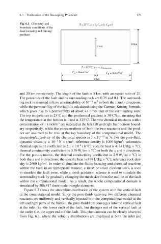
Fig. 6.1 Geometry and T = 25 C, p = 0, C = 0, C = 0
o
boundary conditions of the A B
fluid focusing and mixing
problem

10km

o
T = 325 C, p = α p
1 Hydrostatic
C A = 1kmol /m 3 C B = 1kmol /m 3
20km

and 20 km respectively. The length of the fault is 5 km, with an aspect ratio of 20.
The porosities of the fault and its surrounding rock are 0.35 and 0.1. The surround-
2
ing rock is assumed to have a permeability of 10 –16 m in both the x and y directions,
while the permeability of the fault is calculated using the Carman-Kozeny formula,
which gives rise to a permeability of about 43 times that of the surrounding rock.
The top temperature is 25 C and the geothermal gradient is 30 C/km, meaning that
◦
◦
the temperature at the bottom is fixed at 325 C. The two chemical reactants with a
◦
3
concentration of 1 kmol/m are injected at the left half and right half bottom bound-
ary respectively, while the concentrations of both the two reactants and the prod-
uct are assumed to be zero at the top boundary of the computational model. The
2
dispersion/diffusivity of the chemical species is 3 × 10 –10 m /s. For the pore-fluid,
2
3
dynamic viscosity is 10 −3 N × s/m ; reference density is 1000 kg/m ; volumetric
o
–4
◦
thermal expansion coefficient is 2.1 × 10 (1/ C); specific heat is 4184 J/(kg × C);
o
thermal conductivity coefficient is 0.59 W/(m × C) in both the x and y directions.
o
For the porous matrix, the thermal conductivity coefficient is 2.9W/(m × C) in
o
both the x and y directions; the specific heat is 878 J/(kg × C); reference rock den-
3
sity is 2600 kg/m . In order to simulate the fluids focusing and chemical reactions
within the fault in an appropriate manner, a mesh of small element sizes is used
to simulate the fault zone, while a mesh gradation scheme is used to simulate the
surrounding rock by gradually changing the mesh size from the outline of the fault
within the computational model. As a result, the whole computational domain is
simulated by 306,417 three-node triangle elements.
Figure 6.2 shows the streamline distribution of the system with the vertical fault
in the computational model. Since the pore-fluids carrying two different chemical
reactants are uniformly and vertically injected into the computational model at the
left and right parts of the bottom, the pore-fluid flow converges into the vertical fault
at the inlet (i.e. the lower end) of the fault, but diverges out of the vertical fault at
the outlet (i.e. the upper end) of the fault. This phenomenon can be clearly observed
from Fig. 6.3, where the velocity distributions are displayed at both the inlet and