Page 200 - Fundamentals of Computational Geoscience Numerical Methods and Algorithms

8.2 Some Numerical Simulation Issues Associated with the Particle Simulation Method 191

by n times. Although the one-dimensional idealized particle system is a highly sim-
plified representation of particle models, it illuminates the basic force propagation
mechanism, which is valid for two- and three-dimensional particle models.
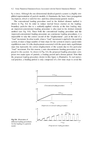
The conventional loading procedure used in the distinct element method is
shown in Fig. 8.6. In order to reduce inertial forces exerted on the loading-
boundary particles due to a suddenly-applied velocity at the first loading step,
an improved-conventional loading procedure is also used in the distinct element
method (see Fig. 8.6). Since both the conventional loading procedure and the
improved-conventional loading procedure are continuous loading procedures, it is
impossible to take the correct record of the “displacement”, just at the end of a
“load” increment. In other words, when a “load” increment is applied to the particle
system, it takes a large number of time steps for the system to reach a quasi-static
equilibrium state. It is the displacement associated with the quasi-static equilibrium
state that represents the correct displacement of the system due to this particular
“load” increment. For this reason, a new discontinuous loading procedure is pro-
posed in this section. As shown in Fig. 8.6, the proposed loading procedure com-
prises two main types of periods, a loading period and a frozen period. Note that
the proposed loading procedure shown in this figure is illustrative. In real numer-
ical practice, a loading period is only comprised of a few time steps to avoid the

V

V=V wall

0 t
(Conventional loading procedure)
V
V=V wall

0 t
t=t full
(Improved conventional loading procedure)
V
V=V wall

Fig. 8.6 Illustration of
different loading procedures 0 t
t=t full
for the loading of a particle
model (Proposed new loading procedure)