Page 208 - Fundamentals of Computational Geoscience Numerical Methods and Algorithms

8.4 Test and Application Examples of the Particle Simulation Method 199

the distinct element method (Zhao et al. 2007b), the proposed upscale theory for the
particle simulation is also approximately valid for the post-failure response of the
particle assembly, as demonstrated in the next section.

8.4 Test and Application Examples of the Particle
Simulation Method

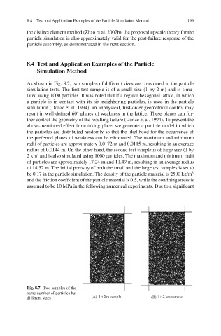
As shown in Fig. 8.7, two samples of different sizes are considered in the particle
simulation tests. The first test sample is of a small size (1 by 2 m) and is simu-
lated using 1000 particles. It was noted that if a regular hexagonal lattice, in which
a particle is in contact with its six neighboring particles, is used in the particle
simulation (Donze et al. 1994), an unphysical, first-order geometrical control may
◦
result in well-defined 60 planes of weakness in the lattice. These planes can fur-
ther control the geometry of the resulting failure (Donze et al. 1994). To prevent the
above-mentioned effect from taking place, we generate a particle model in which
the particles are distributed randomly so that the likelihood for the occurrence of
the preferred planes of weakness can be eliminated. The maximum and minimum
radii of particles are approximately 0.0172 m and 0.0115 m, resulting in an average
radius of 0.0144 m. On the other hand, the second test sample is of large size (1 by
2 km) and is also simulated using 1000 particles. The maximum and minimum radii
of particles are approximately 17.24 m and 11.49 m, resulting in an average radius
of 14.37 m. The initial porosity of both the small and the large test samples is set to
be 0.17 in the particle simulation. The density of the particle material is 2500 kg/m 3
and the friction coefficient of the particle material is 0.5, while the confining stress is
assumed to be 10 MPa in the following numerical experiments. Due to a significant

Fig. 8.7 Two samples of the
same number of particles but
2
different sizes (A) 1× m sample (B) 1× 2 km sample