Page 24 - Fundamentals of Computational Geoscience Numerical Methods and Algorithms

10 2 Simulating Steady-State Natural Convective Problems

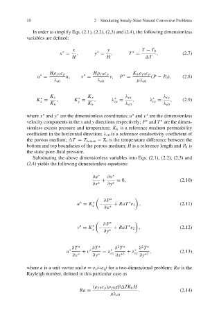
In order to simplify Eqs. (2.1), (2.2), (2.3) and (2.4), the following dimensionless
variables are defined:

x y T − T 0
∗ ∗ ∗
x = , y = , T = , (2.7)
H H ΔT

Hρ f 0 c p Hρ f 0 c p K h ρ f 0 c p
∗ ∗ ∗
u = u, ν = ν, P = (P − P 0 ), (2.8)
λ e0 λ e0 μλ e0

K x K y λ ex λ ey
∗ ∗ ∗ ∗
K = , K = , λ ex = , λ ey = , (2.9)
y
x
K h K h λ e0 λ e0
∗
∗
∗
where x and y are the dimensionless coordinates; u and v are the dimensionless
∗
∗
velocity components in the x and y directions respectively; P and T are the dimen-
∗
sionless excess pressure and temperature; K h is a reference medium permeability
coefficient in the horizontal direction; λ e0 is a reference conductivity coefficient of
the porous medium; ΔT = T bottom − T 0 is the temperature difference between the
bottom and top boundaries of the porous medium; H is a reference length and P 0 is
the static pore-fluid pressure.
Substituting the above dimensionless variables into Eqs. (2.1), (2.2), (2.3) and
(2.4) yields the following dimensionless equations:
∂u ∗ ∂ν ∗
+ = 0, (2.10)
∂x ∗ ∂y ∗

∗
∂ P
∗
∗
u = K ∗ x − + RaT e 1 , (2.11)
∂x ∗
∂ P
∗
∗
∗
v = K y ∗ − + RaT e 2 , (2.12)
∂y ∗
2
2
∂T ∗ ∂T ∗ ∂ T ∗ ∂ T ∗
u ∗ + ν ∗ = λ ∗ ex + λ ∗ ey , (2.13)
∂x ∗ ∂y ∗ ∂x ∗2 ∂y ∗2
where e is a unit vector and e = e 1 i+e 2 j for a two-dimensional problem; Ra is the
Rayleigh number, defined in this particular case as

(ρ f 0 c p )ρ f 0 gβΔTK h H
Ra = . (2.14)
μλ e0