Page 55 - Fundamentals of Computational Geoscience Numerical Methods and Algorithms

3.1 Statement of the Coupled Problem and Solution Method 41

∂σ x ∂τ yx
+ = 0, (3.14)
∂x ∂y
∂τ xy ∂σ y
+ = 0, (3.15)
∂x ∂y
E(1 − v) v EαT
σ x = ε x + ε y − − P, (3.16)

(1 − 2v)(1 + v) 1 − v 1 − 2v
E(1 − v) v EαT
σ y = ε x + ε y − − P, (3.17)

(1 − 2v)(1 + v) 1 − v 1 − 2v
τ xy = τ yx = 2Gγ xy , (3.18)

1
∂u s ∂v s ∂u s ∂v s
ε x = , ε y = , γ xy = + , (3.19)
∂x ∂y 2 ∂y ∂x
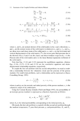
where σ x and σ y are normal stresses of the solid matrix in the x and y directions; ε x
and ε y are the normal strains of the solid matrix in relation to σ x and σ y ; τ xy and γ xy
are shear stress and shear strain of the solid matrix; u s and v s are the horizontal and
vertical displacements of the solid matrix; P is the excess pore-fluid pressure due to

the thermal effect; E and G are the elastic and shear modulus respectively; ν is the
Poisson ratio of the solid matrix and α is the linear thermal expansion coefficient of
the solid matrix.
Note that Eqs. (3.14) and (3.15) represent the equilibrium equations, whereas
Eqs. (3.16), (3.17), (3.18) and (3.19) are the constitutive equations and strain-
displacement relationship equations, respectively.
To couple the first sub-problem with the second sub-problem, we need to estab-
lish a relationship between the volumetric strain and the porosity of the porous
medium. For small strain problems, such a relationship can be expressed as (Itasca
Consulting Group, 1995):

1 − φ 0
φ = 1 − , ε v = ε x + ε y , (3.20)
1 + ε v
where φ and φ 0 are the porosity and initial porosity of the porous medium; ε v is the
volumetric strain of the solid matrix.
Using the Carman-Kozeny formula (Nield and Bejan 1992), the permeability of
an isotropic porous medium is expressed as a function of porosity as follows:

2 3
K 0 (1 − φ 0 ) φ
K x = K y = 3 , (3.21)
φ (1 − φ) 2
0
where K 0 is the initial permeability corresponding to the initial porosity, φ 0 .
Obviously, the first sub-problem is coupled with the second sub-problem through
the medium temperature, T, pore-fluid pressure, p, and permeabilities, K x and K y .