Page 222 - Fundamentals of Ocean Renewable Energy Generating Electricity From The Sea

Ocean Modelling for Resource Characterization Chapter | 8 211

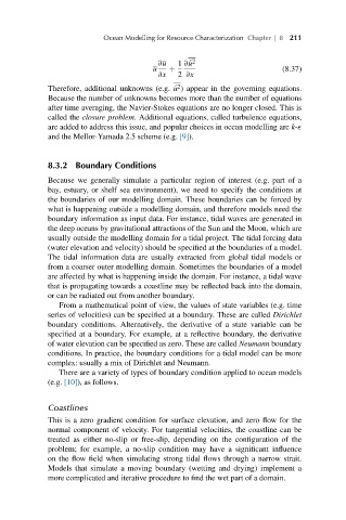
∂u 1 ∂ ´u 2
u + (8.37)
∂x 2 ∂x
2
Therefore, additional unknowns (e.g. ´u ) appear in the governing equations.
Because the number of unknowns becomes more than the number of equations
after time averaging, the Navier-Stokes equations are no longer closed. This is
called the closure problem. Additional equations, called turbulence equations,
are added to address this issue, and popular choices in ocean modelling are k-
and the Mellor-Yamada 2.5 scheme (e.g. [9]).

8.3.2 Boundary Conditions

Because we generally simulate a particular region of interest (e.g. part of a
bay, estuary, or shelf sea environment), we need to specify the conditions at
the boundaries of our modelling domain. These boundaries can be forced by
what is happening outside a modelling domain, and therefore models need the
boundary information as input data. For instance, tidal waves are generated in
the deep oceans by gravitational attractions of the Sun and the Moon, which are
usually outside the modelling domain for a tidal project. The tidal forcing data
(water elevation and velocity) should be specified at the boundaries of a model.
The tidal information data are usually extracted from global tidal models or
from a coarser outer modelling domain. Sometimes the boundaries of a model
are affected by what is happening inside the domain. For instance, a tidal wave
that is propagating towards a coastline may be reflected back into the domain,
or can be radiated out from another boundary.
From a mathematical point of view, the values of state variables (e.g. time
series of velocities) can be specified at a boundary. These are called Dirichlet
boundary conditions. Alternatively, the derivative of a state variable can be
specified at a boundary. For example, at a reflective boundary, the derivative
of water elevation can be specified as zero. These are called Neumann boundary
conditions. In practice, the boundary conditions for a tidal model can be more
complex: usually a mix of Dirichlet and Neumann.
There are a variety of types of boundary condition applied to ocean models
(e.g. [10]), as follows.

Coastlines
This is a zero gradient condition for surface elevation, and zero flow for the
normal component of velocity. For tangential velocities, the coastline can be
treated as either no-slip or free-slip, depending on the configuration of the
problem; for example, a no-slip condition may have a significant influence
on the flow field when simulating strong tidal flows through a narrow strait.
Models that simulate a moving boundary (wetting and drying) implement a
more complicated and iterative procedure to find the wet part of a domain.