Page 47 - Fundamentals of Ocean Renewable Energy Generating Electricity From The Sea

38 Fundamentals of Ocean Renewable Energy

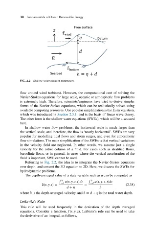
FIG. 2.2 Shallow water equation parameters.

flow around wind turbines). However, the computational cost of solving the
Navier-Stokes equations for large scale, oceanic or atmospheric flow problems
is extremely high. Therefore, scientists/engineers have tried to derive simpler
forms of the Navier-Stokes equations, which can be realistically solved using
available computing resources. One popular simplification is the Euler equation,
which was introduced in Section 2.3.1, and is the basis of linear wave theory.
The other form is the shallow water equations (SWEs), which will be discussed
here.
In shallow water flow problems, the horizontal scale is much larger than
the vertical scale, and therefore, the flow is ‘nearly horizontal’. SWEs are very
popular for modelling tidal flows and storm surges, and even for atmospheric
flow simulations. The main simplification of the SWEs is that vertical variations
in the velocity field are neglected. In other words, we assume just a single
velocity for the entire column of a fluid. For cases such as stratified flows,
baroclinic flows, or in general, in cases where the vertical acceleration of the
fluid is important, SWE cannot be used.
Referring to Fig. 2.2, the idea is to integrate the Navier-Stokes equations
over depth, and convert the 3D equation to 2D. Here, we discuss the SWEs for
hydrodynamic problems.
The depth-averaged value of a state variable such as u can be computed as
η η
−d u(x, y, z, t)dz −d u(x, y, z, t)dz
¯ u(x, y, t) = = (2.38)
d + η h
where ¯u is the depth-averaged velocity, and h = d + η is the total water depth.

Leibnitz’s Rule
This rule will be used frequently in the derivation of the depth averaged
equations. Consider a function, f(x, y, z). Leibnitz’s rule can be used to take
the derivative of an integral, as follows,