Page 439 - Fundamentals of Radar Signal Processing

spectral width is the variance of the spectrum, not the standard deviation.

35. Repeat the spectral width calculation using the version based on the series

approximation to ln(x) given in Eq. (5.113). What is the percentage error in
this estimate compared to the estimate in the previous problem?

36. Assume the simplified target model of Eq. (5.143) and suppose the adaptive
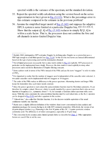
DPCA system is noise limited at a particular Doppler bin, .
Show that the output z[l, k] of Eq. (5.145) reduces to simply Yf [l, k] to
within a scale factor. That is, the processor does not combine the fore and
aft channels in noise-limited Doppler bins.

_____________
1
Skolnik (2001) distinguishes MTI and pulse Doppler by defining pulse Doppler as a system that uses a
PRF high enough to avoid blind speeds (see Sec. 5.2.4). In this text the two terms are instead differentiated
based on the type of processing used and the information obtained.
2
Not all digital processors necessarily form a data matrix similar to Fig. 5.5 explicitly. MTI processors in
particular can be implemented more simply. However, the data matrix is used explicitly in many other
processors and is useful for illustration of Doppler filtering concepts.
3
Some authors work in terms of the PRFs instead of the PRIs and use the term “staggers” to refer to ratios
of PRF .
n
4
It is important to realize that the number of staggers used is independent of the canceller order selected. A
two-pulse canceller can be implemented with two staggers or 10 staggers.
5 The order of the PRIs makes no difference to the power spectrum. Alternating shorter and longer PRIs

keeps the transmitter duty cycle more nearly constant.
6
Since the power spectrum is real-valued, the autocorrelation function must be Hermitian symmetric. It can
therefore be complex valued. However, clutter is usually modeled by a power spectrum that is also an even
function of frequency (i.e., symmetric about F = 0), for example a Gaussian clutter spectrum with a zero
mean. With this extra constraint, the autocorrelation function must be real-valued also, so the Re{} operator
can be dropped in Eq. (5.52) and other equations in this section.
7 “Aliased sinc,” also called the Dirichlet function. It is the discrete-variable equivalent of the usual
continuous-variable sinc function.
8
Harris uses a slightly different definition of the windows than is now conventional in data analysis and
simulation packages for reasons having to do with DFT symmetry properties. Effectively, his version of an
M-point-shaped window (e.g., Hamming) is the first M points of the (M + 1)-point symmetric window
commonly used. The difference is of minor consequence, especially as M gets large.
9
This correction factor assumes pulse-limited ground clutter as described in Chap. 2. Other appropriate
factors are used if this is not the case.