Page 460 - Fundamentals of Radar Signal Processing

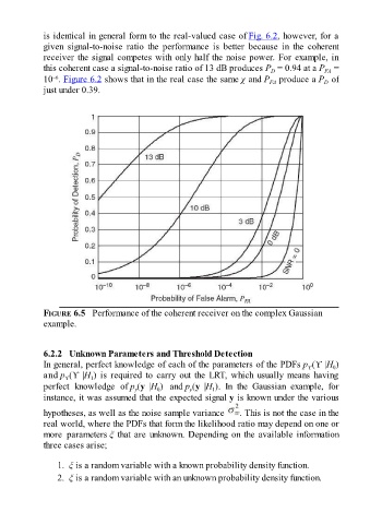
is identical in general form to the real-valued case of Fig. 6.2, however, for a

given signal-to-noise ratio the performance is better because in the coherent
receiver the signal competes with only half the noise power. For example, in
this coherent case a signal-to-noise ratio of 13 dB produces P = 0.94 at a P =
D
FA
–6
10 . Figure 6.2 shows that in the real case the same χ and P produce a P of
D
FA
just under 0.39.

FIGURE 6.5 Performance of the coherent receiver on the complex Gaussian
example.

6.2.2 Unknown Parameters and Threshold Detection
In general, perfect knowledge of each of the parameters of the PDFs p (ϒ |H )
ϒ
0
and p (ϒ |H ) is required to carry out the LRT, which usually means having
ϒ
1
perfect knowledge of p (y |H ) and p (y |H ). In the Gaussian example, for
0
y
1
y
instance, it was assumed that the expected signal y is known under the various
hypotheses, as well as the noise sample variance . This is not the case in the
real world, where the PDFs that form the likelihood ratio may depend on one or
more parameters ξ that are unknown. Depending on the available information

three cases arise;

1. ξ is a random variable with a known probability density function.
2. ξ is a random variable with an unknown probability density function.