Page 14 - Fundamentals of The Finite Element Method for Heat and Fluid Flow

6
B q s d INTRODUCTION

L

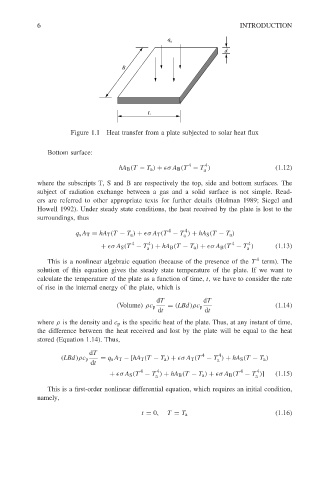
Figure 1.1 Heat transfer from a plate subjected to solar heat flux

Bottom surface:
4
4
hA B (T − T a ) + σA B (T − T ) (1.12)
a
where the subscripts T, S and B are respectively the top, side and bottom surfaces. The
subject of radiation exchange between a gas and a solid surface is not simple. Read-
ers are referred to other appropriate texts for further details (Holman 1989; Siegel and
Howell 1992). Under steady state conditions, the heat received by the plate is lost to the
surroundings, thus
4
4
q s A T = hA T (T − T a ) + σA T (T − T ) + hA S (T − T a )
a
4
4
4
4
+ σA S (T − T ) + hA B (T − T a ) + σA B (T − T ) (1.13)
a
a
This is a nonlinear algebraic equation (because of the presence of the T 4 term). The
solution of this equation gives the steady state temperature of the plate. If we want to
calculate the temperature of the plate as a function of time, t, we have to consider the rate
of rise in the internal energy of the plate, which is
dT dT
(Volume)ρc p = (LBd)ρc p (1.14)
dt dt
where ρ is the density and c p is the specific heat of the plate. Thus, at any instant of time,
the difference between the heat received and lost by the plate will be equal to the heat
stored (Equation 1.14). Thus,
dT 4 4
(LBd)ρc p = q s A T − [hA T (T − T a ) + σA T (T − T ) + hA S (T − T a )
a
dt
4
4
4
4
+ σA S (T − T ) + hA B (T − T a ) + σA B (T − T )] (1.15)
a
a
This is a first-order nonlinear differential equation, which requires an initial condition,
namely,
t = 0, T = T a (1.16)