Page 21 - Fundamentals of The Finite Element Method for Heat and Fluid Flow

13
INTRODUCTION
1.6 Boundary and Initial Conditions
The heat conduction equations, discussed in Section 1.5, will be complete for any prob-
lem only if the appropriate boundary and initial conditions are stated. With the necessary
boundary and initial conditions, a solution to the heat conduction equations is possible.
The boundary conditions for the conduction equation can be of two types or a combination
of these—the Dirichlet condition, in which the temperature on the boundaries is known
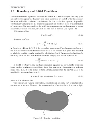
and/or the Neumann condition, in which the heat flux is imposed (see Figure 1.5):
Dirichlet condition

T = T 0 on T (1.46)
Neumann condition
∂T
q =−k = C on qf (1.47)
∂n
In Equations 1.46 and 1.47, T 0 is the prescribed temperature; the boundary surface; n is
the outward direction normal to the surface and C is the constant flux given. The insulated,
or adiabatic, condition can be obtained by substituting C = 0. The convective heat transfer
boundary condition also falls into the Neumann category and can be expressed as

∂T
−k = h(T w − T a ) on qc (1.48)
∂n
It should be observed that the heat conduction equation has second-order terms and
hence requires two boundary conditions. Since time appears as a first-order term, only one
initial value (i.e., at some instant of time all temperatures must be known) needs to be
specified for the entire body, that is,
(1.49)
T = T 0 all over the domain
at t = t 0
where t 0 is a reference time.
The constant, or variable temperature, conditions are generally easy to implement as
temperature is a scalar. However, the implementation of surface fluxes is not as straight-

Γ T Γ qf

Ω

Γ qc

Figure 1.5 Boundary conditions