Page 83 - Fundamentals of The Finite Element Method for Heat and Fluid Flow

75
THE FINITE ELEMENT METHOD
3.3 Formulation (Element Characteristics)
After briefly describing the various elements used in the context of finite element analysis,
we shall now focus our attention on determining the element characteristics, that is, the
relation between the nodal unknowns and the corresponding loads or forces in the form of
the following matrix equation, namely,
[K]{T}={f} (3.169)

where [K] is the thermal stiffness matrix, {T} is the vector of unknown temperatures and
{f} is the thermal load, or forcing vector.
Several methods are available for the determination of the approximate solution to a
given problem. We shall consider three methods in the first instance.
1. Ritz method (Heat balance integral)

2. Rayleigh Ritz method (Variational)

3. Weighted residual methods.
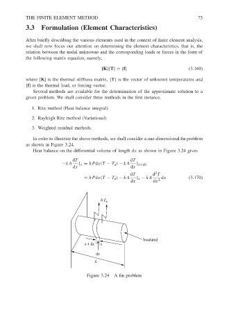
In order to illustrate the above methods, we shall consider a one-dimensional fin problem
as shown in Figure 3.24.
Heat balance on the differential volume of length dx as shown in Figure 3.24 gives

dT dT
−kA | x = hP dx(T − T a ) − kA | x+dx
dx dx
2
dT d T
= hP dx(T − T a ) − kA | x − kA dx (3.170)
dx dx 2

h T a

Insulated
x + dx x
dx
L

Figure 3.24 A fin problem