Page 86 - Fundamentals of The Finite Element Method for Heat and Fluid Flow

78
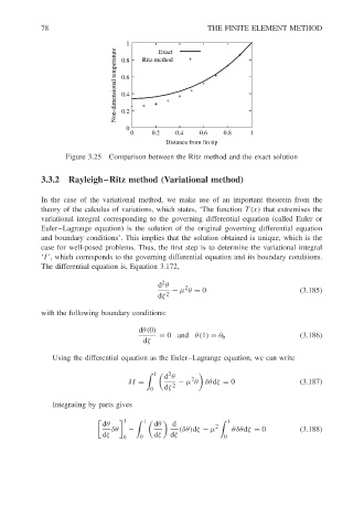
Non-dimensional temperature 0.8 1 Ritz method THE FINITE ELEMENT METHOD
Exact
0.6
0.4

0.2
0
0 0.2 0.4 0.6 0.8 1
Distance from fin tip
Figure 3.25 Comparison between the Ritz method and the exact solution

3.3.2 Rayleigh–Ritz method (Variational method)

In the case of the variational method, we make use of an important theorem from the
theory of the calculus of variations, which states, ‘The function T(x) that extremises the
variational integral corresponding to the governing differential equation (called Euler or
Euler–Lagrange equation) is the solution of the original governing differential equation
and boundary conditions’. This implies that the solution obtained is unique, which is the
case for well-posed problems. Thus, the first step is to determine the variational integral
‘I’, which corresponds to the governing differential equation and its boundary conditions.
The differential equation is, Equation 3.172,

2
d θ 2
− µ θ = 0 (3.185)
dζ 2
with the following boundary conditions:

dθ(0)
= 0and θ(1) = θ b (3.186)
dζ
Using the differential equation as the Euler–Lagrange equation, we can write

2
1 d θ
2
δI = 2 − µ θ δθdζ = 0 (3.187)
0 dζ
Integrating by parts gives

1 1 1
dθ dθ d 2
δθ − (δθ)dζ − µ θδθdζ = 0 (3.188)
dζ dζ dζ
0 0 0